4.3. Modelling and Estimation

The goal is now to:

• estimate parameters of interest (i.e., functional model components of time series) using Best Linear Unbiased Estimation (BLUE);

• evaluate confidence intervals of the estimators for the parameters of interest;

Components of time series

As already discussed, we will distinguish the following components in a time series:

• Trend: General behavior and variation of the process. This often is a linear trend with an unknown intercept \(y_0\) and rate \(r\).

• Seasonality: Regular cyclic variations, which can be expressed as cosine functions with (un)known frequency \(f_1\), and unknown amplitude \(A\) and phase \(\theta\).

• Offset: A jump of unknown size \(o\) in a time series starting at epoch \(t_k\).

• Noise: White or colored noise (e.g., AR process).

Model of observation equations

The linear model, consisting of the above four components, is of the form

\[Y_t = y_0+rt+\underbrace{ a \cos(2\pi f_1t) + b\sin(2\pi f_1t)}_{A \cos(2\pi f_1 t+\theta)}+ou_k(t)+\epsilon(t)\]

The linear model should indeed be written for all time instances \(t_1,...,t_m\), resulting in \(m\) equations as:

\[\begin{split} \begin{align*} Y(t_1) &= y_0+rt_1+a\cos(2\pi f_1 t_1)+b\sin(2\pi f_1 t_1)+ou_k(t_1)+\epsilon(t_1)\\ Y(t_2) &= y_0+rt_2+a\cos(2\pi f_1 t_2)+b\sin(2\pi f_1 t_2)+ou_k(t_2)+\epsilon(t_2)\\ &\vdots \\ Y(t_k) &= y_0+rt_k+a\cos(2\pi f_1 t_k)+b\sin(2\pi f_1 t_k)+ou_k(t_k)+\epsilon(t_k)\\ &\vdots \\ Y(t_m) &= y_0+rt_m+a\cos(2\pi f_1 t_m)+b\sin(2\pi f_1 t_m)+ou_k(t_m)+\epsilon(t_m). \end{align*} \end{split}\]

These equations can be written in compact matrix notation as:

\[Y=\mathrm{Ax}+\epsilon,\]

where

\[\begin{split} \overbrace{\begin{bmatrix} Y_1\\ \vdots\\ Y_{k-1}\\ Y_k\\ \vdots\\ Y_m\end{bmatrix}}^{Y} = \overbrace{\begin{bmatrix} 1&t_1&\cos(2\pi f_1 t_1)&\sin(2\pi f_1 t_1)&0 \\ \vdots&\vdots&\vdots&\vdots&\vdots\\ 1&t_{k-1}&\cos(2\pi f_1 t_{k-1})&\sin(2\pi f_1 t_{k-1})&0\\ 1&t_k&\cos(2\pi f_1 t_k)&\sin(2\pi f_1 t_k)&1\\ \vdots&\vdots&\vdots&\vdots&\vdots\\ 1&t_m&\cos(2\pi f_1 t_m)&\sin(2\pi f_1 t_m)&1\end{bmatrix}}^{\mathrm{A}}\overbrace{\begin{bmatrix}y_0\\ r\\ a\\ b\\ o\end{bmatrix}}^{\mathrm{x}}+\overbrace{\begin{bmatrix}\epsilon(t_1)\\ \vdots\\ \epsilon(t_{k-1}) \\ \epsilon(t_k)\\ \vdots\\ \epsilon(t_m)\end{bmatrix}}^{\epsilon},\end{split}\]

with the \(m\times m\) covariance matrix

\[\begin{split}\Sigma_{Y}=\begin{bmatrix}\sigma_1^2&\sigma_{12}&\dots&\sigma_{1m}\\ \sigma_{21}&\sigma_{2}^2&&\\ \vdots&\vdots&\ddots&\\ \sigma_{m1}&\sigma_{m2}&\dots&\sigma_{m}^2\end{bmatrix}.\end{split}\]

Note that in order to write the model of observation equations as a linear model, we first need to determine frequency \(f_1\).

Exercise

A time series exhibits a linear regression model \(Y(t)=y_0 + rt + \epsilon(t)\). The measurements have also been taken at a measurement frequency of 10 Hz, producing epochs of \(t=0.1,0.2, \dots,100\) seconds, so \(m=1000\). Later an offset was also detected at epoch 260 using statistical hypothesis testing. For the linear model \(Y=\mathrm{Ax}+\epsilon\), establish an appropriate design matrix that can capture all the above effects.

Solution

In the linear regression case, the design matrix consists of two columns, one for the unknown \(y_0\) (a column of ones), and the other for \(r\) (a column of time, \(t\)). Due to the presence of an offset, the mathematical model should be modified to:

\[ Y(t) = y_0 +rt +o_k u_k(t) + \epsilon(t) \]

where \(u_k(t)\) is the Heaviside step function:

\[\begin{split} u_k(t) = \begin{cases} 0, & \textrm{if} & t<t_k=26 \\ 1, & \textrm{if} & t\geq t_k=26 \end{cases} \end{split}\]

and \(o_k\) is the magnitude of the offset. This means that we have to add a third column to the design matrix having zeros before the epoch 260, and ones afterwards. Since epoch 260 corresponds to \(t=26\) s (noting that we have 10 Hz data), in \(\mathrm{A}\) we begin to have 1’s in that row:

\[\begin{split} \mathrm{A} = \begin{bmatrix} 1 & t_1 & 0 \\ \vdots & \vdots & \vdots\\ 1 & t_{259} & 1\\ 1 & t_{260} & 1\\ \vdots & \vdots & \vdots \\ 1 & t_{1000} & 1 \\ \end{bmatrix} = \begin{bmatrix} 1 & 0.1 & 0 \\ \vdots & \vdots & \vdots\\ 1 & 25.9 & 0 \\ 1 & 26 & 1\\ \vdots & \vdots & \vdots \\ 1 & 100 & 1 \\ \end{bmatrix} \end{split}\]

How to find the frequency?

We have seen that to obtain a linear model of observation equations in the presence of a periodic or cyclic pattern (such as seasonality), we need to firstly determine the frequency of the periodic component \(f_1\). Once the frequency is determined, we can construct the design matrix \(\mathrm{A}\). In some applications, the frequency \(f_1\) is provided, while in others, it is not explicitly known and must be estimated from the data.

How to determine \(f_1\) if it is unknown a priori?

We can determine the dominant frequency \(f_1\) by analysing the power spectral density (PSD) of the data. The dominant frequency corresponds to the frequency at which the PSD reaches its maximum value. If the time series contains \(p\) periodic components, the PSD will exhibit \(p\) prominent peaks, one corresponding to each component.

Example power spectral density

Fig. 4.23 shows on the left the original time series as well as the estimated linear trend and seasonal signal. The sine wave has a period (\(T=1/f\)) of 100. Indeed the PSD as function of period on the right shows a peak at a period of 100. Mind that the PSD is shown here as a function of period \(T\) in seconds, rather than frequency \(f\) in Hertz.

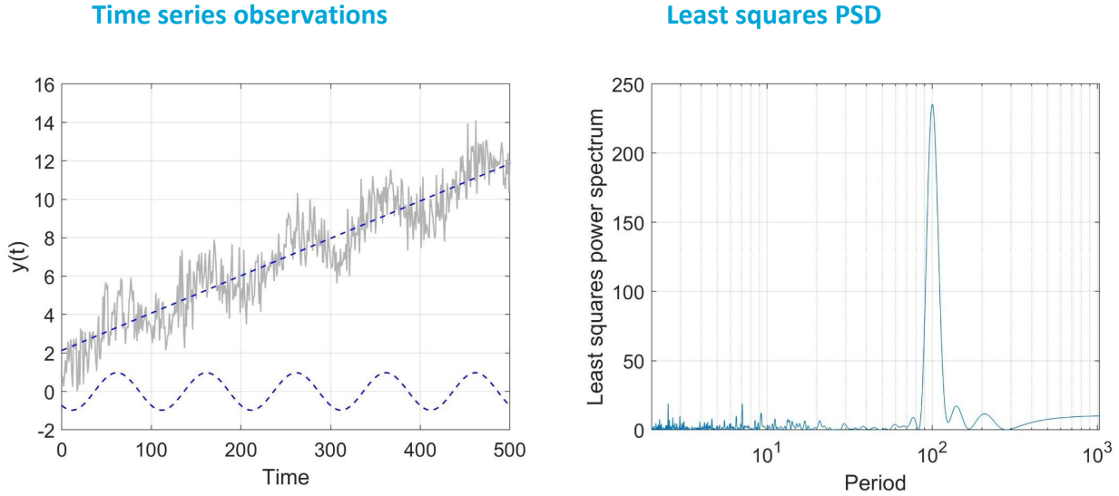
Fig. 4.23 Left: time series (grey) and estimated linear trend and sine wave with period of 100. Right: estimated PSD.

This means we can estimate the frequency \(f_1\) of the periodic pattern using the techniques discussed in the chapter on signal processing. Once we have the frequency, we can construct the design matrix \(\mathrm{A}\).

It is also possible to infer the frequency of the periodic pattern by reasoning. For example, if we know our model depends on temperature, we can assume that the frequency of the seasonal pattern is related to the temperature cycle (e.g., 24 hours). However, this is a more qualitative approach and should be used with caution. Best practice is to use the DFT or PSD to estimate the frequency.

Best Linear Unbiased Estimation (BLUE)

Once the components of time series are known, we may use the linear model of observation equations to estimate those components. We will use the theory from the chapter on observation theory to estimate the parameters of interest.

Consider the linear model of observation equations as

\[Y=\mathrm{Ax}+\epsilon, \hspace{10px} \mathbb{D}(Y)=\Sigma_{Y}\]

Recall that the BLUE of \(\mathrm{x}\) is:

\[\hat{X}=(\mathrm{A}^T\Sigma_{Y}^{-1}\mathrm{A})^{-1}\mathrm{A}^T\Sigma_{Y}^{-1}Y,\hspace{10px}\Sigma_{\hat{X}}=(\mathrm{A}^T\Sigma_{Y}^{-1}\mathrm{A})^{-1}\]

The BLUE of \(Y\) is:

\[\hat{Y}=\mathrm{A}\hat{X},\hspace{10px}\Sigma_{\hat{Y}}=\mathrm{A}\Sigma_{\hat{X}}\mathrm{A}^T\]

and \(\epsilon\) is:

\[\hat{\epsilon}=Y-\hat{Y},\hspace{10px}\Sigma_{\hat{\epsilon}}=\Sigma_{Y}-\Sigma_{\hat{Y}}\]

Note that the BLUE itlself can only be used for prediction when the noise is white and thereby uncorrelated in time (Chapter 4.7).

Estimation of parameters

If we assume the covariance matrix, \(\Sigma_{Y}\), is known, we can estimate \(\mathrm{x}\) using BLUE for the previous example:

\[\begin{split}\hat{X}=\begin{bmatrix}\hat{y_0}\\ \hat{r}\\ \hat{a}\\ \hat{b}\\ \hat{o}\end{bmatrix},\hspace{10px}\Sigma_{\hat{X}}=\begin{bmatrix}\sigma_{\hat{y}_0}^2& \sigma_{\hat{y}_0\hat{r}}& \sigma_{\hat{y}_0\hat{a}}& \sigma_{\hat{y}_0\hat{b}}& \sigma_{\hat{y_0}\hat{o}}\\ \sigma_{\hat{r}\hat{y}_0}& \sigma_{\hat{r}}^2& \sigma_{\hat{r}\hat{a}}& \sigma_{\hat{r}\hat{b}}& \sigma_{\hat{r}\hat{o}}\\ \sigma_{\hat{a}\hat{y_0}}& \sigma_{\hat{a}\hat{r}}& \sigma_{\hat{a}}^2& \sigma_{\hat{a}\hat{b}}& \sigma_{\hat{a}\hat{o}}\\ \sigma_{\hat{b}\hat{y_0}}& \sigma_{\hat{b}\hat{r}}& \sigma_{\hat{b}\hat{a}}& \sigma_{\hat{b}}^2& \sigma_{\hat{b}\hat{o}}\\ \sigma_{\hat{o}\hat{y_0}}& \sigma_{\hat{o}\hat{r}}& \sigma_{\hat{o}\hat{a}}& \sigma_{\hat{o}\hat{b}}& \sigma_{\hat{o}}^2\end{bmatrix}\end{split}\]

Given \(\hat{X}\) and \(\Sigma_{\hat{X}}\), we can obtain the confidence region for the parameters. For example, assuming the observables are normally distributed, a 99% confidence interval for the rate \(r\) is (\(\alpha=0.01\)):

\[\hat{r}\pm k\sigma_{\hat{r}}\]

where \(\sigma_{\hat{r}} = \sqrt{(\Sigma_{\hat{X}})_{22}}\) is the standard deviation of \(\hat{r}\) and \(k=2.58\) is the critical value obtained from the standard normal distribution (using \(0.5\alpha\)).

In many practical applications, the covariance matrix \(\Sigma_{Y}\) is not known. In such cases we can estimate \(\mathrm{x}\) using the unweighted least squares, as then knowledge of the covariance is not needed. Alternatively, it is possible to estimate the variance matrix, or components/parameters of it, based on the observed data through variance component estimation techniques, which are beyond the scope of the MUDE.

Attribution

This chapter was written by Alireza Amiri-Simkooei, Christiaan Tiberius and Sandra Verhagen. Find out more here.