4.1. Discrete events#
Before going further into continuous multivariate distributions, we will start with a reminder of some basic concepts you have seen previously: independence and conditional probability, illustrated by considering the probability of events.
“Set Theory Review: Probability of an Event”
This page is review of a BSc-level probability course. If you need further practice or to revisit other concepts you should refer to the online resource Probability and Statistics for Engineers as needed.
Set Theory Review: Probability of an Event#
In probability theory, the sample space (\(S\)) is the collection of all possible outcomes arising from an experiment or operation which involves chance. An event is the specific outcome, or set of outcomes, from the experiment or operation.
For example, many natural disasters can be considered as binary events: either they occur or don’t occur. This is analogous to flipping a coin, where the ‘flip’ is our experiment and heads or tails define the two possible events. Our sample space is the set of two possible events, where conventionally we will use \(A\) and \(B\) to represent each event, and the probability associated with each is \(P(A)\) and \(P(B)\).
Recall also that the complement of each event is denoted with the “bar” symbol over the top, \(\bar{A}\). This is the probability of event \(A\) not happening and the probability is:
Case Study: discrete events#
Imagine two events, \(A\) and \(B\), where:
\(A\) represents river A flooding
\(B\) represents river B flooding
Each of these events will have a probability of occurring, denoted here as \(P(A)\) and \(P(B)\), respectively, and illustrated in the figure below in the Venn diagram. Recall that the axioms of probability imply that the area of the box represents probability 1.0 (the sample space, \(S\)), and that the shapes in the sample space correspond to probabilities of various events. Based on your understanding of the Venn diagram and probability theory, we can make the following observations from the figure (each statement is provided in layperson terms followed by probability terminology):
Both rivers are flooded at the same time: the probability that \(A\) and \(B\) occur together is not zero (the overlapped area of the circles).
Either river A or B or both rivers are flooded: the probability is the combined area of both circles.
Neither A nor B are flooded: the probability outside (both) circles is not zero
One river is flooded while the other is not: the probability is 1 minus the area of either circle, respectively (i.e., two probabilities, depending on the river, which are not necessarily equal).
These observations and concepts are defined in more detail below.
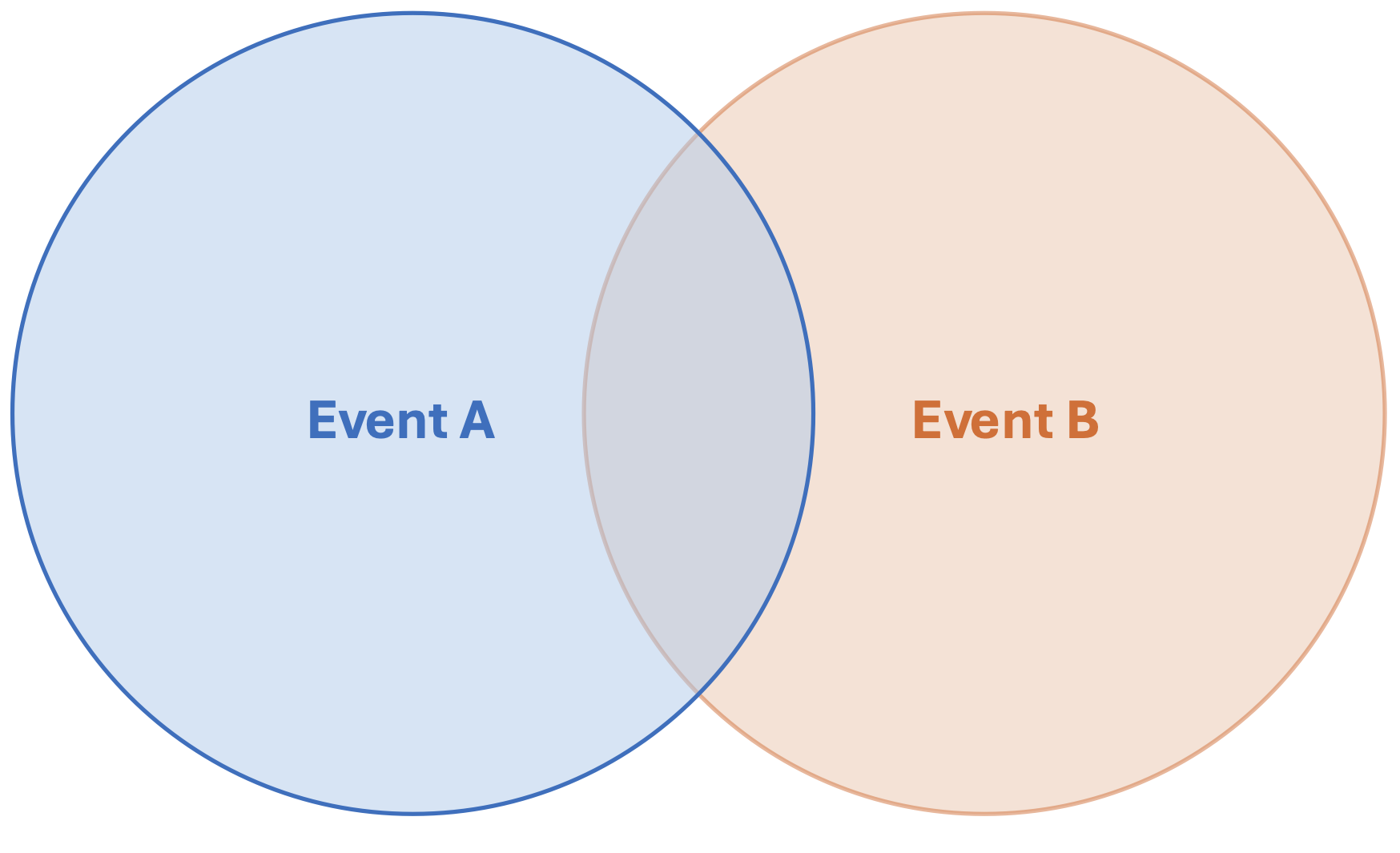
Fig. 4.1 Venn diagram of arbitrary events \(A\) and \(B\).#
Intersection: AND#
The intersection of the events \(A\) and \(B\), denoted \(P(A \cap B)\), is defined as the probability that both events occur; thus, it would be represented in our diagram as shown in the figure below. Going back to our example, it represents the probability that both rivers get flooded at the same time.
The AND probability is the intersection of two events \(P(A \cap B)\).
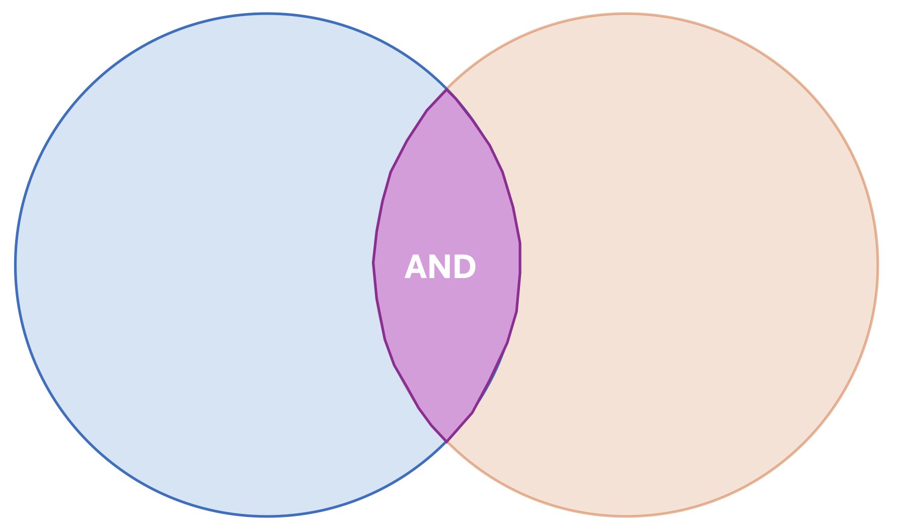
Fig. 4.2 Venn diagram of the events \(A\) and \(B\), and AND probability.#
Union: OR#
The union of events \(A\) and \(B\), \(P(A \cup B)\), is defined as the probability that either either event occurs, or both. In our example, it would represent the probability that either river floods, or both. This probability can be computed as
This is, we add the probabilities of occurrence of the event \(A\) and \(B\) and we deduct the intersection (AND), to avoid counting this area twice. Note that the union is directly related to the intersection of the same events!
The OR probability is the union of two events \(P(A \cup B)\).
Definition of Independence#
When two events, \(A\) and \(B\) are independent, it means that the occurrence of one does not influence the occurrence of the other. Formally, \(A\) and \(B\) are considered independent if and only if the AND probability (\(P(A \cap B)\)) can be factorized into the product of their probabilities. That is:
As long as we know the probabilities of each event the computation of the AND probability is a simple multiplication problem. This simplicity is why the assumption of independent events is often invoked.
Although the assumption of independence makes our modelling and programming efforts more simple, it is often not a good representation of reality; improving our ability to model these situations is the primary motivation for this chapter, which will provide alternative methods for computing \(P(A \cap B)\).
Tip
The primary purpose of this chapter is to facilitate the computation of the AND probability for dependent events and dependent random variables (the next page), which can be simply described as the case:
Conditional probability#
A conditional probability describes the probability of an event given that another event is known to have occurred.
where \(P(A|B)\) is the probability of the event \(A\) given that event \(B\) is known to have occurred. Note that when reading the equation the vertical bar \(|\) is read out loud as “given,” and identifies the combination of events \(A|B\) as “\(A\) conditioned on \(B\).”
The concept can be illustrated graphically by recognizing that once \(B\) is known to have occurred, it’s probability is now 1.0 and the task at hand is to determine the probability of \(A\). Using the figure above, this is equivalent to taking the area of the circle \(B\) as the new sample space and noting the probability \(P(A)\) is given by the fraction of the circle where \(A\) is overlapped: the intersection, \(P(A \cap B)\). As the probability of \(B\) is now 1.0, we must scale \(P(A \cap B)\) proportionally (normalizing by \(P(B)\)), thus arriving at the equation above: simple!
Conditional Probability of Independent Events#
What happens to the conditional probability if the events are independent?
Thus, the probability of \(A\) given \(B\) is simply the probability of \(A\).
When \(A\) and \(B\) are independent the probability of \(A\) is not influenced by the probability of \(B\).
This can be interpreted graphically by recognizing that the area of the overlapped area of events \(A\) and \(B\) is equivalent to the product of the area of the individual circles.
Tip
It is common to confuse mutually exclusive events with independent events. The former states that two events cannot happen simultaneously, which implies that \(P(A|B)=P(A)P(B)=0\), whereas the latter dictates how the AND probability can be computed (and generally speaking \(P(A|B)\) is not 0, although it can be).
Refer to the reference probability book for a refresher, if needed.
Although the definition above is illustrated with a simple case of two discrete events, it is essential to remember it when working with more complicated situations, for example multivariate probability distributions for continuous random variables.
Total probability theorem#
When the probability of an event cannot be calculated directly, but its occurrence is related to the occurrence of other events, the Total probability theorem can be applied as
where \(B_i\) are a set of mutually exclusive and collectively exhaustive events. This result can also be derived graphically using a Venn diagram with multiple events in the sample space.
If you need further refresher of these concepts, you can further read and practice here.
Attribution
This chapter was written by Patricia Mares Nasarre and Robert Lanzafame. Find out more here.