1. Extreme Value Analysis#
Attribution
This chapter was written by Patricia Mares Nasarre. Find out more here.
The preceding chapters have focused on a variety of data-driven and physics-based modelling techniques which we primarily used to interpolate between known data (e.g., machine learning), or make predictions about phenomena where randomness did not play a significant role (e.g., finite volume or finite element methods applied to simple physics problems). Most of the methods and problems considered ignored (or greatly simplified) the stochastic nature of the underlying processes. When uncertainty was considered explicitly, it focused primarily on error and epistemic types, for example, the inclusion of various types of noise in Time Series Analysis, or measurement precision in Observation Theory. In these cases, the focus was on applications that were governed by variations around a central value (as opposed to the tails of the distribution), which are often modelled sufficiently using a Gaussian distribution.
The chapter on Continuous Distributions introduced additional asymmetric parametric distributions, such as the Gumbel or Exponential, which are better able to represent the observations that have a small frequency in a data set (i.e., rare events). Regardless of their flexibility, these distributions are not possible to validate for cases where data simply does not exist, which is where concepts introduced in this chapter become useful.
Continuous parametric distributions are relatively simple models to apply, and allow one to make inferences of values of the modelled random variable that occur infrequently, or not at all, within the available observations (i.e., the data set) due to a key concept: the tail of the distribution. When extrapolating to values outside a set of observations, fitting of the parametric distribution to the tail is crucial to provide a reasonable extrapolation. Consider the following figure, which was covered earlier in this book:
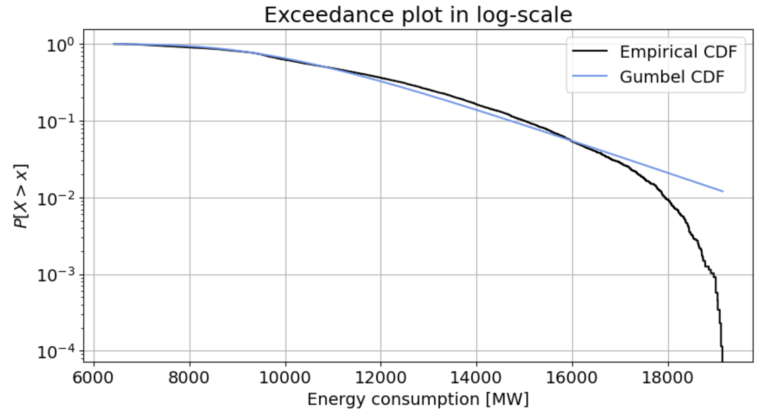
Fig. 1.13 Exceedance plot in semi-log scale comparing a continuous parametric distribution to data of energy consumption. Note in particular the divergence between data and model above 16,000 MW, or below probability of exceedance of 0.06.#
In the example above right-tailed Gumbel distribution was fit to observations on energy consumption, where the Gumbel distribution was selected to represent the positive skewness (right tail) present in the data. While the behavior around the central moments was well represented, the tail was not properly modelled, which is visible in the divergence between data and model on the right-hand side of the plot.
But what happens if my main interest is the tail?
In many engineering applications there is typically an interest in the tails of the distributions. For instance, flood protection systems will be designed to withstand extreme rainfall events or extreme river discharges (low exceedance probabilities), not only daily conditions (high exceedance probabilities); these extreme events are located in the tails of the distribution. Moreover, by definition, extreme events are typically scarce in our datasets, as they occur infrequently. The available time series are usually short (e.g., 20 years) in comparison with the design events that the system needs to withstand (e.g., 1,000 years event).
Extreme Value Analysis (EVA) focuses on those events located at the tails of the distribution (extreme events) and provides a framework to identify and model the stochastic behavior of these extreme events such that events which have not been observed can be inferred.
In the following chapters, the formal concept of extreme will be introduced, as well as the techniques to sample them, without data, and probabilistically model them.
We will cover two methods of performing an extreme value analysis: block maxima and peak over threshold, both of which are applied in the same way:
Identify a random variable of interest that can be modelled with a continuous parametric probability distribution
Prepare and explore the data set that will be used to fit a distribution
Sample the data to collect a set of the extreme observations
Fit a distribution to the sampled set of data
Repeat the sampling and fitting process as needed, evaluating the alternatives, until a suitable model is identified
As you can see above, only step 3 is a significant departure from what was covered earlier in the continuous distribution chapters.
MUDE exam information
You are expected to understand the general motivation of extreme value analysis and be able to use it to choose and use an appropriate distribution for making inferences about a random variable of interest. It is important to know the key steps of the methods in general (for example, the sampling process), as well as the differences and advantages/disadvantages of block maxima and peak over threshold approaches.
Boxes such as this are used throughout the chapters to indicate where specific theory is provided only as background information (i.e., not required for the exam).
At the end of these chapters you can also find supplementary videos that cover the same material as the book (although there is not a 1-to-1 relationship between pages and videos).