3.2. Least-squares estimation

Functional model: dealing with inconsistency

Given a set of observations which contain noise, and a model that is assumed to explain these data, the goal is to estimate the unknown parameters of that model. The least-squares principle can be used to solve this task.

Mathematically, we use the ‘system of observation equations’, with the \(m\)-vector of observations \(\mathrm{y}\), the \(n\)-vector of unknowns \(\mathrm{x}\), and the \(m \times n\) design matrix \(\mathrm{A}\). In a simple form, we can write this system of observation equations as

\[ \mathrm{y = Ax}. \]

If all the observations would fit perfectly to this model, this system is called consistent. This is only possible if the number of observations \(m\) is equal to (or smaller than) the number of unknowns \(n\), i.e. if the system is determined.

If the number of observations is greater than the number of unknowns (and the design matrix \(\mathrm{A}\) is of full column rank), it is very unlikely that the system is consistent. Physical reality would need to be perfectly described by the conceptual mathematical model. It is evident that in real life this is never the case, since (i) our observations are always contaminated by some form of noise, and (ii) physical reality is often more complex than can be described with a simplified mathematical model.

Thus, in the case in which there are more observations than unknowns (and design matrix \(\mathrm{A}\) is of full column rank) the \(\mathrm{y=Ax}\) system of equations has no solution, this is referred to as an overdetermined system. In other words; every ‘solution’ would be wrong, since the model would not perfectly ‘fit’ the data.

The redundancy of the system is equal to \(m-n\), i.e., the ‘additional’ number of observations compared to the minimum required to solve the system of equations.

Example: linear trend model

Assume we have \(m\) observations and we try to fit the linear trend model:

\[\begin{split} \begin{bmatrix} y_1 \\ y_2 \\ \vdots \\ y_m \end{bmatrix} = \underset{\mathrm{A}}{\underbrace{\begin{bmatrix} 1 & t_1 \\ 1 & t_2  \\ \vdots & \vdots \\ 1 & t_m \end{bmatrix}}}\underset{\mathrm{x}}{\underbrace{\begin{bmatrix} x_1 \\ x_2 \end{bmatrix}}} \end{split}\]

Fig. 3.4 shows the observations, together with a fitted linear trend line. Obviously, it is impossible to fit a line that perfectly matches all observations due the small measurement errors, which are assumed to be random.

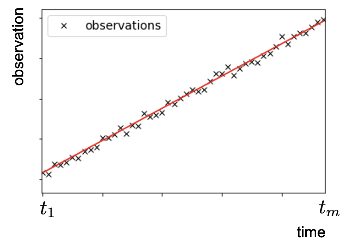
Fig. 3.4 Linear trend line fitted to a set of \(m\) observations affected by random errors.

We solve the problem of having an ‘unsolvable’ equation by considering the random errors for each observation:

\[ \mathrm{y=Ax + \epsilon} \]

The length of the error vector (or vector of residuals) \(\mathrm{\epsilon}\) is equal to the length of the vector of observations \(\mathrm{y}\).

Least-squares principle

We are looking for a solution for \(\mathrm{x}\); this solution will be denoted by \(\hat{\mathrm{x}}\). Based on this solution, the ‘adjusted observations’ would be \(\hat{\mathrm{y}}= \mathrm{A}\hat{\mathrm{x}}\) (solution of the forward model).

To find a solution for an inconsistent system of equations, we prefer the one for which the observations are ‘as close as possible’ to the model. This is a ‘minimum distance’ objective. In mathematical terms, we look at the vector of residuals \(\hat{\epsilon}\): the difference between the observations \(\mathrm{y}\) and the model realization \(\mathrm{\hat{y}}\):

\[ \mathrm{\hat{\epsilon}=y-\hat{y}=y-A\hat{x}} \]

We want this vector of residuals to be as small as possible (i.e., the minimum distance objective). The ‘least-squares’ principle achieves this by minimizing (‘least’) the sum of the squared residuals (‘squares’).

If we take the square-root of this sum, we find the length of the vector, also known as the norm of the vector. Thus, the various possible error vectors have a norm defined as:

\[ \left \| \epsilon \right \| = \sqrt{\epsilon_1^2+\epsilon_2^2+...+\epsilon_m^2}=\sqrt{\epsilon^T\epsilon} \]

Finding the minimum of (a) the sum of the squared differences, or (b) the square-root of the sum of the squared differences, yields the same result, since both terms are always positive or zero.

If we find this minimum, the corresponding solution \(\mathrm{\hat{x}}\) is the least-squares solution of the system of observation equations. In mathematical terms this is written as

\[ \mathrm{\hat{x}} = \arg \underset{\mathrm{x}}{\min} \left \| \epsilon \right \|^2= \arg \underset{x}{\min} {(\epsilon^T\epsilon)} \]

From the system observation equations \(\mathrm{y=Ax+\epsilon}\), it follows directly that \(\epsilon=\mathrm{y-Ax}\) and therefore the least-squares solution follows as:

\[ \mathrm{\hat{x}} =\arg \underset{\mathrm{x}}{\min} {\mathrm{(y-Ax)^T (y-Ax)}}. \]

In other words, \(\mathrm{\hat{x}}\) is the solution for \(\mathrm{x}\) which provides the minimum of \(\mathrm{(y-Ax)^T (y-Ax)}=\sum_{i=1}^m \epsilon_i^2\), hence the smallest sum of squared residuals.

Least-squares solution

We can find the minimum of a function by taking the first derivative with respect to the ‘free variable’. Since the observation vector is not free, and also the design matrix \(\mathrm{A}\) is fixed, the only variable which we can vary is \(\mathrm{x}\). The first derivative of our objective function should be equal to zero to reach a minimum (see Gradient, and Vectors and matrices):

\[\begin{split} \begin{align*} \partial_x \mathrm{(y-Ax)^T (y-Ax)} &=0\\ \partial_x \left(\mathrm{ y^T y -(Ax)^T y -y^T Ax + (Ax)^T (Ax)} \right)&=0\\ \partial_x \mathrm{( y^T y -x^T A^T y -y^T Ax + x^T A^T Ax )}&=0\\ \partial_x \mathrm{(y^T y -2x^T A^T y + x^T A^T Ax) }&=0\\ \mathrm{-2A^T y + 2A^T Ax} &=0\\ \mathrm{A^T Ax} &=\mathrm{A^T y } \end{align*} \end{split}\]

This last equation is known as the normal equation, and the matrix \(\mathrm{N=A^T A}\) is known as the normal matrix.

MUDE exam information

You will not be asked to derive the least-squares solution as above.

If it is possible to compute the inverse of the normal matrix, the normal equation can be written to express the estimate of \(\mathrm{x}\), denoted by \(\mathrm{\hat{x}}\), as a linear function of the observations:

\[ \mathrm{\hat{x}= (A^T A)^{-1} A^T y} \]

Summary

In summary, the least-squares estimates of \(\mathrm{x}\), \(\mathrm{y}\) and \(\epsilon\) are given by:

\[ \mathrm{\hat{x}= (A^T A)^{-1} A^T y} \]

\[ \mathrm{\hat{y} = A \hat{x}} \]

\[ \mathrm{\hat{\epsilon} = y - A\hat{x} = y - \hat{y}} \]

Fig. 3.5 visualizes the least-squares solution based on a linear trend model.

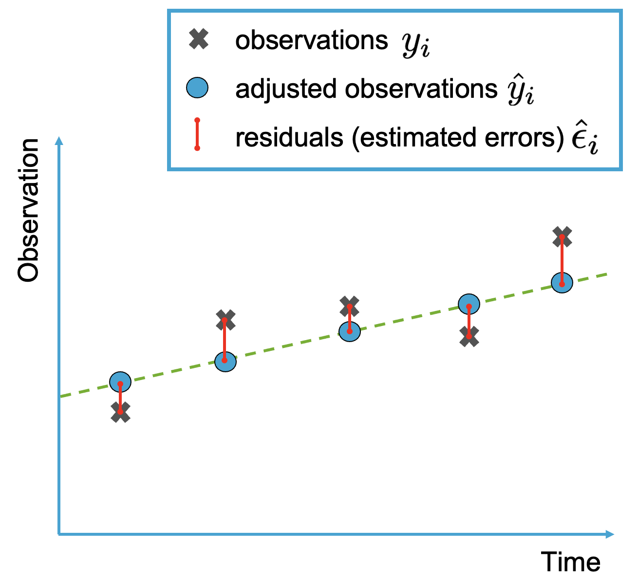
Fig. 3.5 Least-squares fit to a set of 5 observations affected by random errors. Index \(i\) refers to the \(i\)th observation.

Attribution

This chapter was written by Sandra Verhagen. Find out more here.