5.4. Example Linear Programming#
Videos#
The story is told in two videos. The videos have a one-to-one correspondence with this book
The sand and clay extraction problem#
Solving the sand and clay extraction problem with the graphical solution method#
The problem#
A company extracts sand and clay from a site which when sold gives a profit of 57 and 60 monetary units per thousand units of product, respectively. For this extraction, sand needs a manpower of 50 workers x hours to extract 1000 units of product whilst clay needs 13 workers x hours for 1000 units.
4 hours of backhoe are needed to extract one thousand units of sand and 5 hours of backhoe work per thousand units of clay. The number of hours needed of truck transport is 8h and 4h, respectively for sand and clay for each 1000 units of product transported.
The company has a work schedule of 40 hours per week for the workers but also for the equipment (truck and backhoe). There are 5 workers who can be used interchangeably between the transport of the two products. There is only one truck and one backhoe.
Main questions:
What should be the extraction plan of this company in a week?
What should their objective be?
What decisions need to be made?
LP formulation of the problem#
\(x_1\) - thousands of units of sand to be produced and transported in one week
\(x_2\) - thousands of units of clay to be produced and transported in one week
Our objective function then will look like (with \(L\) being the profit in monetary units for one week):
subject to:
\(8x_1+4x_2\leq 40\): maximum number of hours of the vehicle driving time per week
\(4x_1+5x_2\leq 40\): maximum number of hours of crane work per week
\(50x_1+13x_2\leq 200\): maximum of 5 (workers) x 40 hours of driving time available per week per worker
\(x_1,x_2\geq 0\): the production must be positive!
Solution#
The above mentioned constraints define the feasible region of the solution space. The feasible region is represented by the yellow polygon on the graph below:
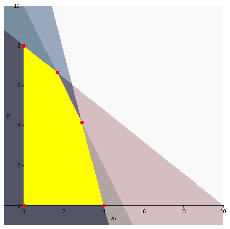
The regions at green, blue, and red correspond to the first three constraints defined in the previous subsection, in the same order. The yellow region is a result of the super position of these three regions alongside \(x_1\geq 0\) and \(x_2\geq 0\). All the points inside and in the border of the yellow region are solutions for our problem!
How can we find the optimal solution now?
Our solution space, in this case, is a closed polygon, which is always convex in LP problems (it is easily seen in the graph represented above that any line connecting two points inside our solution space is always inside the polygon).
Theorem
The set of feasible solutions is a convex set whose extremes (vertices) correspond to feasible basic solutions. If there is, at least, a feasible solution to the problem, then there is a feasible basic solution to the problem.
If the objective function has a finite maximum (minimum) there is at least an optimal solution and that is a feasible basic solution (one of those vertices).
We consider as basic solutions any of the red vertices of the yellow region, and any other solution that is inside the highlighted yellow region consists of a non-basic solution.
To find the optimal solution, we can start now by computing the gradient vector of the objective function whose direction gives us the direction of growth of the objective function, i.e.:
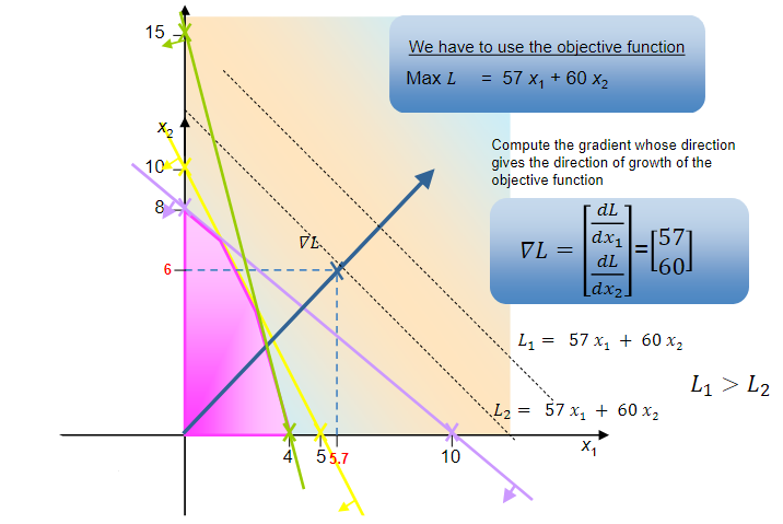
With this, we just need to find the last point inside the feasible region in the direction of the gradient (maximization) or the first point inside the region (minimization). That point will be one of the vertices (basic solutions), and in this example we get:
If we calculate the value of the objective function for the remaining vertices we confirm that the one we obtained above consists in the one that maximizes \(L\):
\(\mu_1=(0,8)\implies L=480\)
\(\mu_2=\left(\frac{35}{12},\frac{25}{6}\right)\implies L = 416.5\)
\(\mu_3=(4,0)\implies L=228\)
\(\mu_4=(0,0)\implies L=0\)
Attribution
This chapter is written by Gonçalo Homem de Almeida Correia, Maria Nogal Macho, Jie Gao and Bahman Ahmadi. Find out more here.