3.5. Precision and confidence intervals

When evaluating and reporting estimation results, it is important to give a quality assessment. Thereby we should distinguish between:

• the precision of the estimated parameters (topic of this part)

• how well the model fits the data (topic of chapter Model testing)

The precision of the estimated parameters is provided by the covariance matrix \(\Sigma_{\hat{X}}\). But the question is: how to present and interpret the numbers in the matrix? For that purpose we will introduce the concept of confidence intervals, which basically means we will ‘convert’ the precision to probabilities.

Video

Review normal distribution and probabilities

Let’s start with a standard normally distributed random variable \(Z\sim N(0,1)\), which has an expectation equal to 0, and standard deviation (for us: precision) of 1. Fig. 3.6 shows the corresponding PDF.

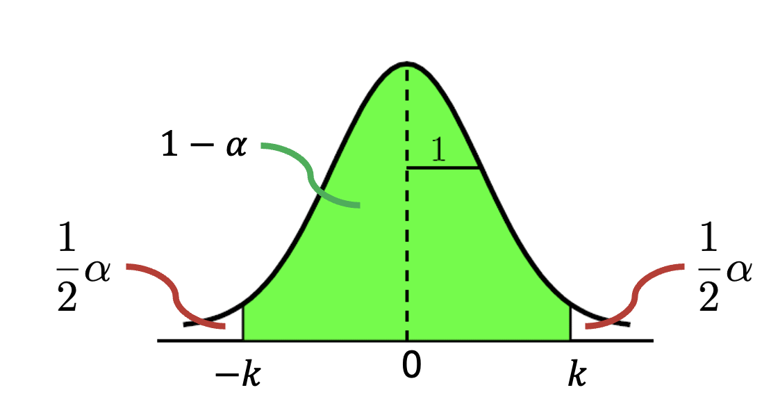
Fig. 3.6 PDF of standard normally distributed random variable.

We are now interested in the probability that a realization of \(Z\) will be within a certain interval \(\pm k\) from the expectation 0:

\[ P(-k<Z<k) = P(|Z|<k) = 1-\alpha \]

In this case, \(k\) is the \((1-0.5\alpha)\)-quantile, since it can be seen in Fig. 3.6 that

\[ P(Z<k) = 1-0.5\alpha \]

If we choose a certain value for \(\alpha\) we can thus find the value of \(k\) using the inverse CDF, e.g., with \(\alpha = 0.05\) we would obtain \(k=1.96\), see Table Standard Normal distribution (note that you would have to look up the value for 0.025 in the table).

Confidence interval of observations

Definition

A confidence interval of a random variable \(\epsilon \sim N(0,\sigma_{\epsilon}^2)\) is defined as the range or interval \(\epsilon \pm c\) such that:

\[ P(|\epsilon|<c) = 1-\alpha \]

where \((1-\alpha)\cdot\) 100% is the confidence level.

On purpose we considered \(\epsilon \sim N(0,\sigma_{\epsilon}^2)\) in the above definition, since in observation theory we generally assume that the random errors in our observations are normally distributed with zero mean and variance \(\sigma^2_{\epsilon}\).

Similarly as for the standard normal distribution, the interval \(\pm c\) can be computed. We will do this by first applying the transformation:

\[ \frac{\epsilon - 0}{\sigma_{\epsilon}} = Z \sim N(0,1) \]

With this we have that:

\[ P(|\epsilon|<c) = P(|\frac{\epsilon}{\sigma_{\epsilon}}|<\frac{c}{\sigma_{\epsilon}})= P(|Z|< k) \]

with \(c = k\sigma_{\epsilon}\).

This allows us to compute \(k\) as shown in Review normal distribution and probabilities and express the confidence interval as:

\[ \epsilon \pm k\sigma_{\epsilon} \]

For example, for a confidence level of 95% we have \(\alpha = 0.05\), for which we found \(k=1.96\). Hence the corresponding confidence interval is \(\epsilon \pm 1.96\sigma_{\epsilon}\).

So far we considered the confidence level of a single random error. If we have multiple observations, the corresponding intervals can be evaluated. Even though the precision of each observation may be different, we only need to compute \(k\) once to find the intervals \(\epsilon_i \pm k\sigma_{\epsilon_i}\), \(i=1,\ldots,m\).

Fig. 3.7 shows how the confidence intervals can be visualized as error bars for the corresponding observations \(y_i\).

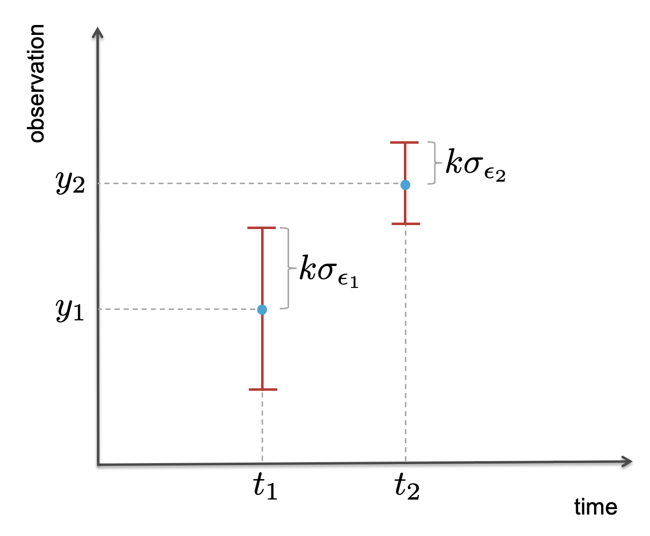
Fig. 3.7 Confidence intervals of two observations \(y_1\) and \(y_2\) visualized with error bars.

Note

The error bars in Fig. 3.7 should not be interpreted as the interval such that there is \(1-\alpha\) probability that the true value of \(Y_i\) is in that interval. We are namely only looking at a single realization of each \(Y_i\), while the confidence interval is computed based on the probability that the random error deviates \(\pm k\sigma_{\epsilon_i}\) from 0, and hence that \(Y_i\) deviates by that amount from its expected value. If we would repeat the two measurements, the values of \(y_1\) and \(y_2\) will be different and hence the error bars would be shifted.

Confidence intervals of estimated parameters

The covariance matrix \(\Sigma_{\hat{X}}\) of a linear estimator can be evaluated by applying the linear propagation law of covariances. Moreover, we know that if our observables \(Y\) are normally distributed, applying linear estimation implies that the estimated parameters \(\hat{X}\) are also normally distributed. Recall that the weighted least-squares and Best Linear Unbiased estimators are indeed linear estimators.

The covariance matrices of the BLUE estimator were obtained as:

\[\begin{split} \begin{align*} \Sigma_{\hat{X}}&=(\mathrm{A^T} \Sigma_Y^{-1} \mathrm{A})^{-1}\\ \Sigma_{\hat{Y}}&= \mathrm{A}\Sigma_{\hat{X}} \mathrm{A^T} \\ \Sigma_{\hat{\epsilon}}&=\Sigma_Y-\Sigma_{\hat{Y}} \end{align*} \end{split}\]

Following the same logic as above, the confidence intervals for each estimated parameter can be evaluated as:

\[\begin{split} \begin{align*} \hat{x}_i &\pm k\sigma_{\hat{X}_i} \\ \hat{y}_i &\pm k\sigma_{\hat{Y}_i} \\ \hat{\epsilon}_i &\pm k\sigma_{\hat{\epsilon}_i} \\ \end{align*} \end{split}\]

where \(k\) is determined by the chosen confidence level.

Fig. 3.8 shows a visualization of the confidence interval of the predicted observations, i.e., the fitted model.

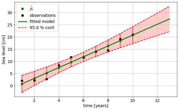
Fig. 3.8 Confidence interval of fitted model, including error bars for the individual adjusted observations \(\hat{y}_i\).

Note that covariance matrices can be computed without the need for actual observations. Hence, we can also set up a functional model including future epochs (add extra rows to the original design matrix \(\mathrm{A}\)). Let’s call the corresponding design matrix \(\mathrm{A_p}\), then \(\Sigma_{\hat{Y}_p}= \mathrm{A_p}\Sigma_{\hat{X}} \mathrm{A_p^T}\). Note that the \(\Sigma_{\hat{X}}\) is based on the original model, since the fitted model is only based on the actual observations. In this way, we can visualize the uncertainty of extrapolated values based on the fitted model.

Factors influencing the precision

As can be seen from the expression \(\Sigma_{\hat{X}}=(\mathrm{A^T} \Sigma_Y^{-1} \mathrm{A})^{-1}\), the precision of the estimates depends on the:

• design matrix \(\mathrm{A}\): proper design of the measurement set-up can improve the precision

• covariance matrix \(\Sigma_Y\): more precise observations will result in more precise estimates

Not immediately clear from the expression is that also the redundancy (\(=m-n\)) is an important factor: more observations will improve the precision, due to the averaging of the random errors (if \(m\) large enough, the mean error will go to zero).

Exercise uniform motion

Attribution

This chapter was written by Sandra Verhagen. Find out more here.