Components of time series

import numpy as np
import matplotlib.pyplot as plt
%matplotlib inline

Introduction:

The four components of time series, we will consider here, are the trend, seasonality, offset, and noise (white/colored). We use simulated data to show these components here. The observation equation of time series should have the following mathematical representation:

\[Y(t) = y_0 + r t + a \cos(\omega_0t) + b\sin(\omega_0t) + o {u_k(t)} + \epsilon(t)= y_0 + r t + A \cos(\omega_0 t+\phi_0) + o {u_k(t)} + \epsilon(t)\]

where

• \(y_0 \): intercept (e.g. in mm)

• \(r\): is the rate (e.g. in mm/day)

• \(a\) and \(b\) are the coefficients of the periodic signal

• \(\omega_0\) is the frequency of signal (e.g. cycle/ day)

• \(o\) is the size of the offset at time instant \(t_k\)

• \(u_k(t)\) is the unit step function which is 1 if \(t_k \leq t\) and 0 otherwise

• \(\epsilon(t)\) is the random noise with a given variance which follows a Normal distribution: \( \epsilon(t) \sim \textbf{N}(0, \sigma^2)\)

Here, we are assuming only a single seasonality and offset component. However, in many practical scenarios, there could be multiple components related to these.

Exercise:

You can simulate your time series based on the priori information provided in the scripts. Plot your results and change the input variables to see the effect.

The noise follows a normal distribution: use np.random.normal in order to draw random samples from a normal (Gaussian) distribution. Study more for this function here.

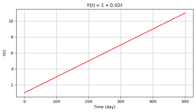
We will first create the time series \(Y(t)=y_0+rt\), with \(y_0=1\) mm and \(r=0.02\) mm/day with a duration of 500 days (i.e., time series consists of 500 observations).

np.random.seed(0)  # For reproducibility

time = np.arange(501) 
m = len(time)
y_0 = 1 
r = 0.02 
y1 = y_0 + r*time 

plt.figure(figsize=(8,4))
plt.grid()
plt.plot(time, y1, color='red')
plt.ylabel('Y(t)')
plt.xlabel('Time (day)')
plt.title('$Y(t) = 1 + 0.02 t $');

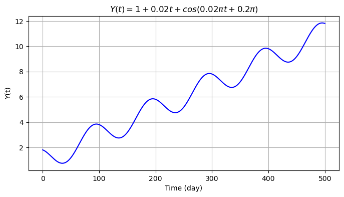
We then introduce seasonality to the data with a cosine signal \(s(t)=A \cos(\omega_0 t + \phi_0)\) with \(\omega_0=2\pi f\), frequency \(f=0.01\) cycle/day (i.e., 1 cycle per 100 days), amplitude \(A=1\) mm and initial phase \(\phi_0=0.2\pi\) rad.

omega_0 = 2 * np.pi/100 
A = 1 
phi_0 = 0.2*np.pi 
y2 = y1 + A*np.cos(omega_0 * time + phi_0) 

plt.figure(figsize=(8,4))
plt.grid()
plt.plot(time, y2, color='blue')
plt.ylabel('Y(t)')
plt.xlabel('Time (day)')
plt.title('$Y(t) = 1 + 0.02 t + cos(0.02πt + 0.2π)$');

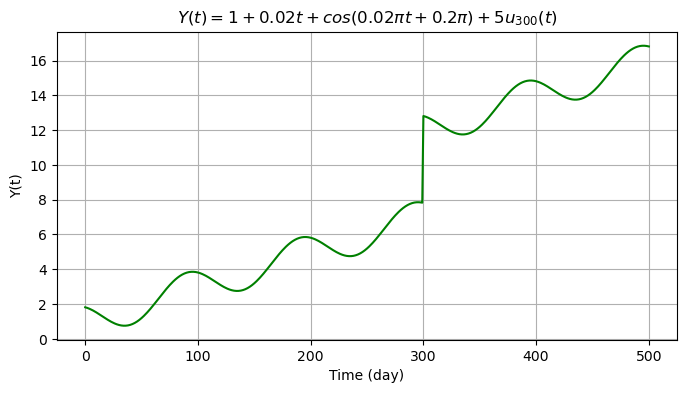
We now add an offset \(o_k=5\) at \(t=300\) days. We therefore create a copy of the previous signal and store it into a new array.

t_k = 300 
O_k = 5 
y3 = y2.copy() 
y3[t_k:] = y3[t_k:] + O_k

plt.figure(figsize=(8,4))
plt.grid()
plt.plot(time, y3, color='g')
plt.ylabel('Y(t)')
plt.xlabel('Time')
plt.title('$Y(t) = 1 + 0.02 t + cos(0.02πt + 0.2π) + 5 u_{300}(t)$');

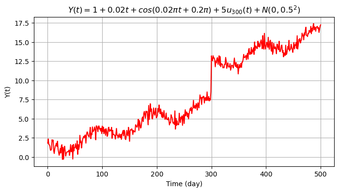
Eventually we include the random error \(\epsilon \sim \textbf{N}(\mu, \sigma_e)\) with \(\mu=0\) mm and \(\sigma_e=0.5\) mm.

mean = 0 
sigma = 0.5 
et = np.random.normal(loc = mean, scale = sigma, size = m) 
y4 = y3 + et 

plt.figure(figsize=(8,4))
plt.grid()
plt.plot(time, y4, color='red')
plt.ylabel('Y(t)')
plt.xlabel('Time')
plt.title('$Y(t) = 1 + 0.02 t + cos(0.02πt + 0.2π) + 5 u_{300}(t) + N(0,0.5^2)$');

Attribution

This chapter was written by Alireza Amiri-Simkooei, Christiaan Tiberius and Sandra Verhagen. Find out more here.