5.2. Empirical Distributions

As you can imagine, it is possible to define a PDF and a CDF based on observations. Let’s see it with an example dataset of wind speeds close to Schiphold Airport. The figure below shows the dataset which spans for 1 year.

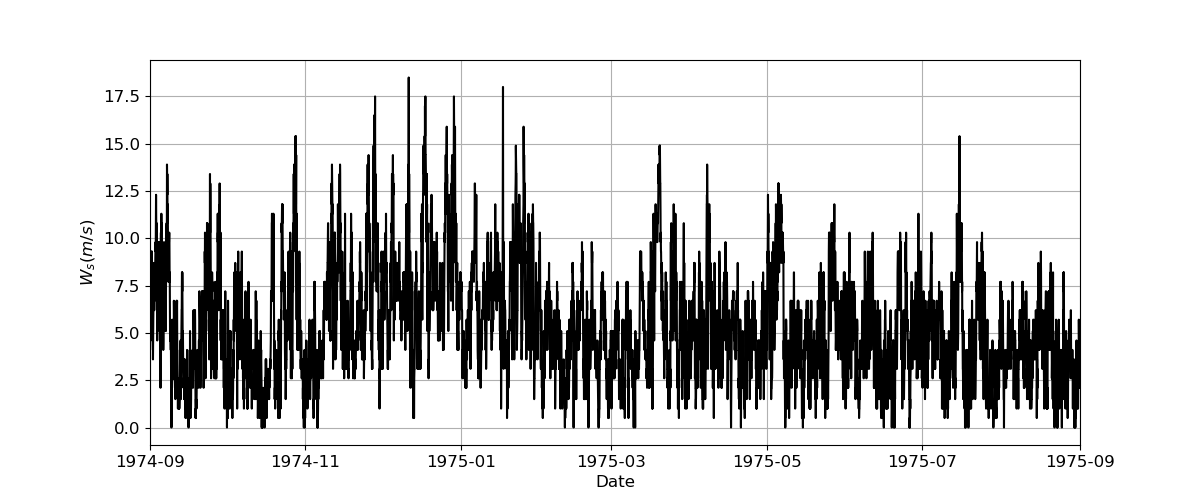
Fig. 5.5 Time series of wind speed close to Schiphol Airport.

Let’s start computing the empirical CDF. We need to assign to each observation a non-exceedance probability. To do so, we just need to sort the observations and compute the non-exceedance probabilities using the ranks. This is illustrated below with pseudo-code.

read observations

x = sort observations in ascending order

length = the number of observations
probability of not exceeding = (range of integer values from 1 \
                                to length) / length + 1

plot x versus probability of not exceeding 

Using the above algorithm, the following figure is obtained. Note that empirical CDFs are usually plotted using a step plot.

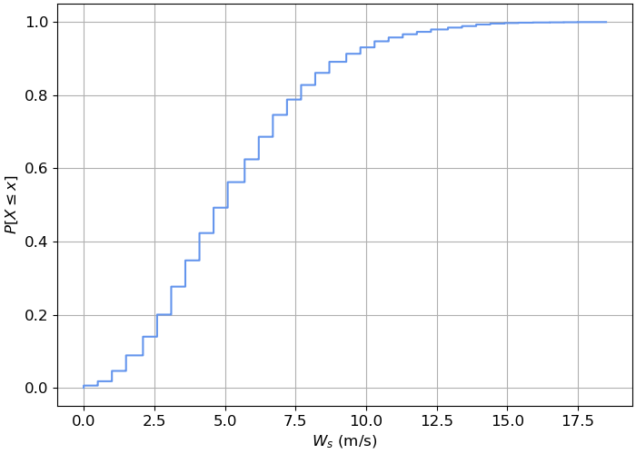
Fig. 5.6 Empirical cumulative distribution function of the wind speed data.

It can be useful to also visualize the empirical PDF. As mentioned above, the PDF is the derivative of the CDF, leading to the following equation.

\[ f(x) = F'(x) = \lim_{\Delta x \to 0} \frac{F(x+\Delta x)-F(x)}{\Delta x} \]

Thus, we can compute the empirical PDF assuming a bin size. To do so, we need to count the number of observations in each bin and calculate the relative frequency of each bin by dividing that count with the total number of observations. The density will be then those relative frequencies divided by the bin size. This process is illustrated with the following pseudo-code 1.

read observations

#Assume the bin size
bin_size = 2

#Calculate the number of bins and the bin edges given the bin size
min_value = minimum value of observations
max_value = maximum value observations 
n_bins = (max_value - min_value) / bin_size 
bin_edges = range of n_bins + 1 values between the truncated value \
            of min_value and the ceiling value of max_value

#Count the number of observations in each bin
count = empty list
for each bin:
    append the number of observations between the bin_edges to count

#Compute relative frequencies
freq = count / number of observations

#Compute densities
densities = freq / bin_size

#plot epdf
barplot densities

Using the above algorithm, the following figure is obtained. We can see that most of the density is concentrated between 2 and 9 m/s.

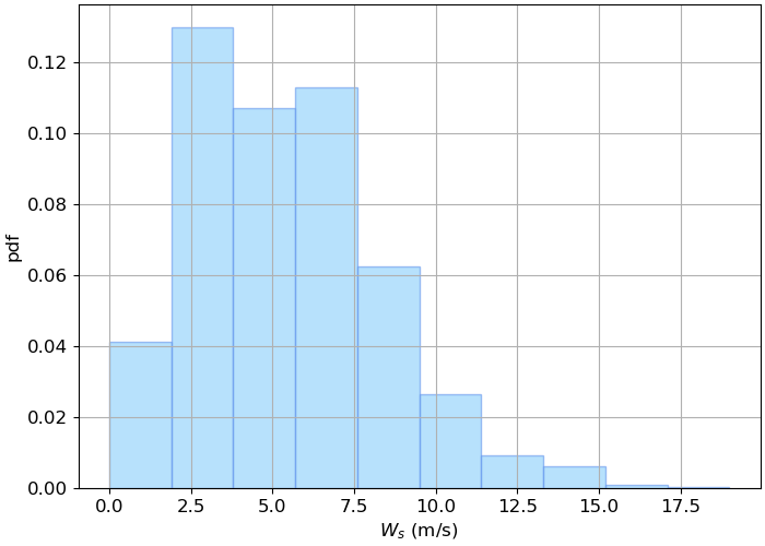
Fig. 5.7 Empirical probability density function of the wind speed data.

Attribution

This chapter was written by Patricia Mares Nasarre and Robert Lanzafame. Find out more here.

---

1

Happily, in most coding languages, the algorithm to compute the pdf is already implemented and we just need to plot a histogram selecting the option to show us the densities.