3.3. Fourier Transform#
Before starting…#
Let us start by taking a look into the results found in the previous chapter. We have defined the complex exponential Fourier series for a periodic signal \(x(t)\) as:
with \(\omega_0=2\pi f_0\) and \(k\in\mathbb{Z}\) and complex coefficients found as
where the integration period \(T_0\) is taken symmetrically about zero.
Fourier Transform#
When the period \(T_0\) increases, the frequencies belonging to the Fourier series coefficients (\(kf_0\)) lie closer and closer together as \(f_0=1/T_0\) decreases. Now, what if \(T_0\) approaches infinity? That is, what would happen if we have an a-periodic signal?
Fourier coefficients will lie infinitesimally close to each other, so they define continuous function of frequency, \(f\approx kf_0\)

MUDE Exam Information
This derivation is provided for additional insight and will not be part of the exam.
Substituting the definition of the series coefficients into \(x(t)\), we find
Now, when \(T_0\to\infty\), \(f_0\) becomes infinitesimally small, \(f_0\to df\). Multiplying \(f_0\) with \(k\) then becomes a continuous function, \(kf_0\to f\). The summation from \(k=-\infty\) to \(k=\infty\) then becomes an integration in \(f\) from \(f=-\infty\) to \(f=\infty\)
Re-arranging the terms:
The integral between parentheses is defined as Fourier integral or (continuous-time) Fourier transform, \(\mathcal{F}()\):
The complex number \(X_k\) of the Fourier series is now a complex function of the frequency, \(f\): \(X(f)\).
The inverse Fourier transform, \(\mathcal{F}^{-1}()\) can also be derived
Note
To obtain \(x(t)\) from \(X(f)\), we integrate over frequency, \(f\), and the result is a function of time, \(t\)
Hence, Fourier transform and its inverse can be used to transform time signal to the frequency domain, and the other way around. This yields a Fourier transform pair:
Conditions#
Sufficient conditions for convergence of Fourier transform integrals are:
\(x(t)\) absolutely integrable, i.e. \(\int_{-\infty}^{\infty}|x(t)|dt<\infty\)
discontinuities, if any, should be finite
Amplitude and phase#
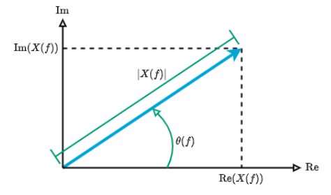
Like the coefficients of complex Fourier series, a Fourier transform can also be written in terms of magnitude and phase:
with
When \(x(t)\) is real, we have \(X(f)=X^*(-f)\), and then
Magnitude \(|X(f)|\) is an even function of \(f \to\) amplitude spectrum
Phase \(\theta(f)\) is an odd function of \(f \to\) phase spectrum
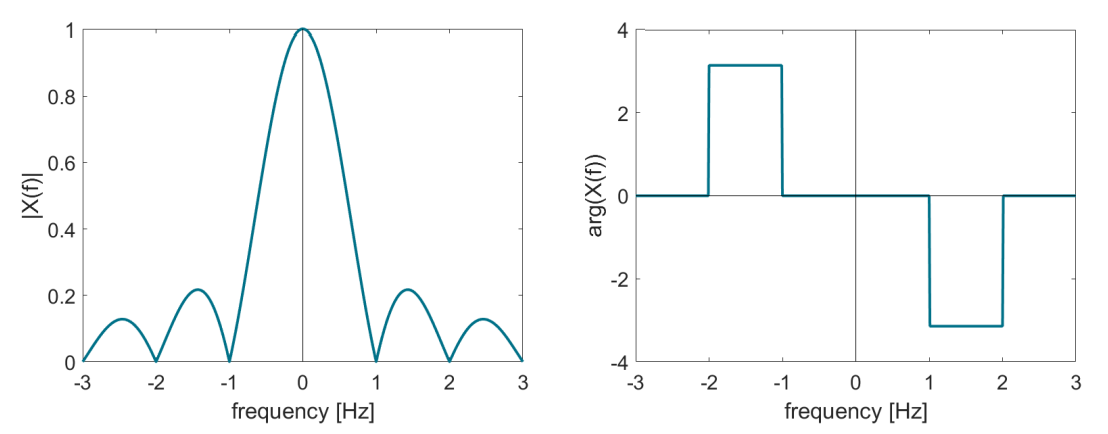
The figure above illustrates an example of \(|X(f)|\) and \(\theta(f)\) both as a function of frequency.
Summary#
A-periodic functions can be written as integrals, continuous over frequency. This yields the so-called Fourier transform (and its inverse):
Amplitude and phase spectrum are given by:
Exercises#
The signal \(x(t)=\Pi(\frac{t}{\tau})\) is defined by a pulse function with duration \(\tau\) [s]:
Derive an expression for the Fourier transform \(X(f)\) of signal \(x(t)\).
Hint: you may want to use Euler’s formula to turn the difference of two complex exponentials into a sine function. In addition, to turn your answer into an even more compact form, you may want to use the cardinal sine, which is defined as \(\textrm{sinc}(z)=\frac{\sin(\pi z)}{\pi z}\).
Solution
The video below illustrates how to arrive at the final solution, which is presented here:
The solution can also be found using SymPy:
import sympy as sym
t = sym.symbols('t')
tau, f = sym.symbols('tau, f', positive=True)
x = sym.Piecewise((0, t < -tau/2), (1, t < tau/2), (0, True))
display(x)
\(\begin{cases} 0 & \rm{for}\: t < - \frac{\tau}{2} \\1 & \rm{for}\: t < \frac{\tau}{2} \\0 & \rm{otherwise} \end{cases}\)
solution = sym.integrate(x*sym.exp(-sym.I*2*sym.pi*f*t), (t,-sym.oo,sym.oo))
simplified_solution = sym.simplify(solution)
display(solution)
display(simplified_solution)
\(- \cfrac{i e^{i \pi f \tau}}{2 \pi f} + \cfrac{i e^{- i \pi f \tau}}{2 \pi f}\)
\(\cfrac{\sin{\left(\pi f \tau \right)}}{\pi f}\)
Given the Fourier transform \(X(f)=\delta(f)\), find the expression for signal \(x(t)\). Then, verify the following two points:
When \(x(t)=e^{j2\pi f_0 t}\), then \(X(f)=\delta(f-f_0)\), and
When \(x(t)=\cos(2\pi f_0 t)\), then \(X(f)=\frac{1}{2}(\delta(f-f_0)+\delta(f+f_0))\).
Hint: for the first part (finding \(x(t)\)), use the inverse Fourier transform, and use the sifting property of the Dirac delta function (in this case in the frequency domain) when solving the integral.
Solution
The video below illustrates how to arrive at the final solution, which is presented here:
Attribution
This chapter is written by Christiaan Tiberius. Find out more here.