
import matplotlib
if not hasattr(matplotlib.RcParams, "_get"):
    matplotlib.RcParams._get = dict.get
6.5. Feedforward Neural Networks#
# pip install packages that are not in Pyodide
%pip install ipympl==0.9.3
%pip install seaborn==0.12.2
# Import the necessary libraries
import numpy as np
import matplotlib.pyplot as plt
from sklearn.neural_network import MLPRegressor
from sklearn.preprocessing import StandardScaler
from mude_tools import neuralnetplotter, draw_neural_net
from cycler import cycler
import seaborn as sns

%matplotlib widget

# Set the color scheme
sns.set_theme()
colors = [
    "#0076C2",
    "#EC6842",
    "#A50034",
    "#009B77",
    "#FFB81C",
    "#E03C31",
    "#6CC24A",
    "#EF60A3",
    "#0C2340",
    "#00B8C8",
    "#6F1D77",
]
plt.rcParams["axes.prop_cycle"] = cycler(color=colors)
This page contains interactive python element: click –> Live Code in the top right corner to activate it.
Introduction#
Recall that in the previous chapters we have applied linear models with basis functions
Here \(\mathbf{w}\) are the flexible parameters, and \(\boldsymbol{\phi}\) the basis functions.
Because a linear model is linear in its parameters \(\mathbf{w}\), we could solve for \(\bar{\mathbf{w}}\) directly
where \(\mathbf{\Phi}\) is the collection of basis functions evaluated in all data points. The basis functions need to be chosen a priori for this approach. When the phenomenon to be modeled is complex, relying on pre-defined basis functions might not give sufficient accuracy. We can overcome this issue with a more flexible model. Aside from the pragmatic strategy of increasing the number of basis functions, we can also achieve more flexibility by replacing the basis functions with parametric functions. In this chapter we will dive into one variant of this concept, namely neural networks. The underlying problem will stay the same: we are trying to learn a process based on a limited number of noisy observations \(\mathcal{D}=\{\mathbf{X}, \mathbf{t}\}\). Following decision theory, we need to minimize the mean squared error loss function
where \(y(x, \mathbf{w})\) now comes from a neural network.
# The true function relating t to x
def f_truth(x, freq=2, **kwargs):
    # Return a sine with a frequency of f
    return np.sin(x * freq)


# The data generation function
def f_data(epsilon=0.7, N=100, **kwargs):
    # Apply a seed if one is given
    if "seed" in kwargs:
        np.random.seed(kwargs["seed"])

    # Get the minimum and maximum
    xmin = kwargs.get("xmin", 0)
    xmax = kwargs.get("xmax", 2 * np.pi)

    # Generate N evenly spaced observation locations
    x = np.linspace(xmin, xmax, N)

    # Generate N noisy observations (1 at each location)
    t = f_truth(x, **kwargs) + np.random.normal(0, epsilon, N)

    # Return both the locations and the observations
    return x, t
Neural network architecture#
A neural network consists of neurons connected by weights, with information flowing from input neurons towards output neurons. In supervised learning, the states of the input and output neurons are known during training. There are additional neurons in layers in between the inputs and outputs, forming a so-called hidden layer. Neurons are separated into layers, where all neurons of one layer depend on (at least) the neurons of the previous layer.
The state of a neuron is determined by a linear combination of states \(z\) from the previous layer with their connecting weights \(w\)
where \(w_{j0}^{(l)}\) are so-called biases, allowing the model to have an offset. Make sure not to confuse this quantity with the model bias from the bias-variance tradeoff discussion. This linear combination of states is followed by a nonlinear transformation with an activation function \(h(\cdot)\):
In the plot below, we can see the identity (or linear), sigmoid, hyperbolic tangent (tanh), and rectified linear unit (relu) activation functions applied on an arbitrary state \(z\) in the \([-4,4]\) range.
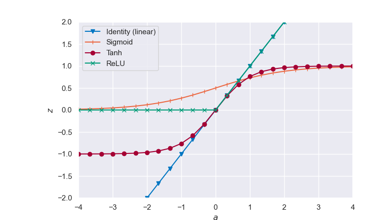
Fig. 6.32 Activation functions#
The number of layers in a neural network commonly refers to the number of hidden layers. Following the aforementioned setup of compounding linear transformations with nonlinear activations, the output of a two-layer neural network can be written as:
Since the activation function can be nonlinear and quantities proportional to the weights pass through them, the model is evidently no longer necessarily linear w.r.t. the weights and, in general, no closed-form Maximum Likelihood solution can be found. Compare this with the linear basis function models from before. Instead of seeking an analytical solution that no longer exists, some sort of gradient-based optimization scheme, as discussed in the previous chapter in the form of SGD, is required calibrate the weights.
When your dataset contains multiple inputs or outputs, this model can easily be extended by including multiple neurons in the input or output layer, and the other procedures stay the same. Generally, the activation function of the outputs \(h^{(out)}\) is linear and the activations in hidden layers are of a nonlinear type.
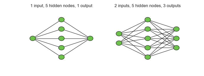
Fig. 6.33 Two neural networks#
Coding neural nets
Feedforward neural networks are often also called Multilayer Perceptrons (MLP) in machine learning software packages. This is also the case for scikit-learn, the package you will be using during the workshop this week. In that package, a neural network model for regression can be instantiated by using the MLPRegressor class.
Refer to the documentation of scikit-learn to see which arguments you can pass when creating a new MLPRegressor. These include the number of layers in the network, the number of units in each layer, the type of activation function, etc.
Model flexibility#
The flexibility of a feedforward neutral network can be adapted by varying the number of neurons per hidden layer, or by adding more hidden layers. Both options lead to an increase in the number of parameters \(\mathbf{w}\). When a neural network has too few parameters, it generally puts us at risk of underfitting the data, whereas having too many parameters can quickly lead to overfitting. Since they control model complexity, the number of layers and neurons per layer are therefore hyperparameters, which need to be calibrated. Once again, remember that hyperparameters are calibrated with validation data. Simply minimizing training error w.r.t. these hyperparameters will always lead to huge and severely overfit models, especially when we do not have a lot of data available.
Coding neural nets
It is usual to perform a so-called grid search when performing model selection for models with more than one hyper-parameter. The strategy is to train a separate model for each combination of hyperparameters and pick the one with the lowest value for validation loss. Conceptually, code for this could look something like:
hp1vals = [val1, val2, ...]
hp2vals = [val1, val2, ...]
val_losses = np.zeros(len(hp1vals),len(hp2vals))

for i, hp1 in enumerate(hp1vals):
    for j, hp2 in enumerate(hp2vals):
        # build the model
        model = Model(hp1,hp2)

        # train the model
        lowest_val_loss = train_model(model, X_train, t_train, X_val, n_epochs)

        # store loss
        val_losses[i,j] = lowest_val_loss

# pick model with lowest entry in val_losses
In the following interactive plot you can study the influence of the number of neurons per layer on model prediciton. The number of hidden layers is fixed at two. You have to click the re-run button to retrain the model after varying the parameter. Be aware that the required computations can take a few moments to run. Hide the table of contents to see the full image.
# Define the prediction locations
# (note that these are different from the locations where we observed our data)
x_pred = np.linspace(-1, 2 * np.pi + 1, 200)

xscaler = StandardScaler()
xscaler.fit(f_data()[0][:, None])


# Function that creates a NN
def NN_create(**kwargs):
    return MLPRegressor(
        solver="sgd",
        hidden_layer_sizes=(kwargs["neurons"], kwargs["neurons"]),
        activation=kwargs["activation"],
        batch_size=kwargs["batch_size"],
    )


# Function that trains a given NN for a given number of epochs
def NN_train(x, t, network, epochs_per_block):
    # Convert the training data to a column vector and normalize it
    X = x.reshape(-1, 1)
    X = xscaler.transform(X)

    # Run a number of epochs
    for i in range(epochs_per_block):
        network.partial_fit(X, t)

    return network, network.loss_curve_


# Function that returns predictions from a given NN model
def NN_pred(x_pred, network):
    # Convert the prediction data to a column vector and normalize it
    X_pred = x_pred.reshape(-1, 1)
    X_pred = xscaler.transform(X_pred)

    # Make a prediction at the locations given by x_pred
    return network.predict(X_pred)
# Pass everything to the neuralnetplotter
plot1 = neuralnetplotter(
    f_data,
    f_truth,
    NN_create,
    NN_train,
    NN_pred,
    x_pred,
    N=100,
    val_pct=60,
    epochs=20000,
)
plot1.fig.canvas.toolbar_visible = False
plot1.add_sliders("neurons", valmax=20, valinit=3)
plot1.add_buttons("truth", "seed", "reset", "rerun")
As you might have noticed, using the default setting of three neurons per layer was not enough for the network to learn the underlying trend in the data. Which number of neurons per layer gave you a visibly good fit? Did you ever spot overfitting?
Pay close attention to what we show on the right-hand plot during training:
Line color |
Quantity |
Expression |
|---|---|---|
Blue |
Training set loss (\(40\%\) of \(N\)) |
\(E_D=\frac{1}{N_\mathrm{train}}\sum_{n=1}^{N_\mathrm{train}} \left(t_n - y(x_n, \mathbf{w}) \right)^2\) |
Purple |
Validation set loss (\(60\%\) of \(N\)) |
\(E_D=\frac{1}{N_\mathrm{val}}\sum_{n=1}^{N_\mathrm{val}} \left(t_n - y(x_n, \mathbf{w}) \right)^2\) |
Black |
Expected loss (numerical integration) |
\(\mathbb{E}[L]=\int\int\left(t-y(x,\mathbf{w})\right)^2p(x,t)dxdt\) |
The black line is a very precise version of our error, but one that requires a lot of data to obtain. Since analytical integration is not possible due to the complex nature of \(t\) and \(y(x,\mathbf{w})\), we are forced to compute it through numerical integration, in this case by using \(1500\) equally-spaced predictions in the range \([0,2\pi]\). Although interesting to include here for educational purposes, it is obvious that we will not have access to this measure in practice.
What we have instead is the validation loss (purple line) computed as a relatively crude Monte Carlo approximation of the expected loss, since we are only using a very small number of data points to compute it. In practice, we need to rely on this approximation to make model selection decisions!
Coding neural nets
As with any other model this week, we need to perform a training-validation-test split to our original dataset in order to arrive at a robust machine learning estimator for \(y(x)\). A simple (incomplete) implementation of this procedure could look like:
import numpy as np

# fix the seed of the RNG, for reproducibility
np.random.seed(42)

# get an index array with randomized order
perm = np.random.permutation(N)

# compute the number of samples for training/validation/test
n_train = ...
n_val = ...
n_test = ...

# slice the permutation vector from before
idcs_train = perm[0:ntrain]
idcs_val = perm[...:...]
idcs_test = perm[...:...]

# use the indices to slice X and t
X_train = X[idcs_train]
t_train = t[idcs_train]
# ...
Early stopping#
Choosing a high number of neurons increases the number of parameters and, therefore, slows down training. In addition, it can make the model too flexible and prone to overfitting. It is therefore good practive to always monitor the predictive capability of a NN on a validation set. First, run the model below, then, select the model you think best fits the data by pulling the corresponding slider. At which epoch do you find the best model?
plot2 = neuralnetplotter(
    f_data,
    f_truth,
    NN_create,
    NN_train,
    NN_pred,
    x_pred,
    neurons=20,
    epochs=12000,
    N=40,
    val_pct=60,
    batch_size=2,
)
plot2.fig.canvas.toolbar_visible = False
plot2.seed = 4
plot2.add_sliders("cur_model")
plot2.add_buttons("truth", "seed", "reset", "rerun")
plot2.show()
The example above is a good illustration of overfitting. Note how the training loss almost immediately becomes an unreliable estimate of the true expected loss (black line). In contrast, the validation loss (purple line) does not exactly agree with the black line but consistently follows the same trends. Crucially, the validation loss correctly points to the model with the lowest true loss, at around \(3000\) training epochs. Move the model selection slider there and try to see why the true loss starts to increase from that point on.
It is possible to train a neural network for a long time, and then select the \(\mathbf{w}\) that corresponds to the lowest validation error. An alternative, known as early stopping, uses the indication that the validation loss increases for a number of epochs as a stopping sign to halt training.
Coding neural nets
To make early stopping work, we need to continuously monitor the validation loss, either every time the model is updated or at least once every epoch. Together with the fact that we train with mini-batches of our dataset (as explained in the video), this means we need to code a training loop that implements our SGD routine.
In scikit-learn we could call the fit function to fully train a network. However, in order to properly implement early stopping, keep track of our validation loss and see which mini-batches are being picked, we could code our own training loop. To accommodate for this, the MLPRegressor model offers the partial_fit function, that retrains the network only once for a given pair of X_batch and t_batch. Then one possible (incomplete) implementation could look like:
def train_model(model, X_train, t_train, X_val, n_epochs):
    for epoch in range(n_epochs):
        # slice the dataset into mini-batches
        batches = slice_dataset(X_train,t_train)

        for X_batch, t_batch in batches:
            # update network weights
            model.partial_fit(X_batch, t_batch)

        # compute the relevant losses
        train_y = model.predict(X_train)
        val_y   = model.predict(X_val)

        train_loss = loss_function(train_t,train_y)
        val_loss = loss_function(val_t,val_y)

        # append losses to the relevant lists
        t_losses.append(train_loss)
        v_losses.append(val_loss)
    return t_losse, v_losses
where care should be of course taken to properly normalize the datasets. The losses can then be plotted, the model with the best validation loss can be picked, etc.
Manual model selection#
In Linear Basis Function Models and Regularization we used L2-regularization to control the model complexity. The application of this technique to neural networks is straightforward, and will therefore not be demonstrated here. Instead, we will focus on the impact of the number of trainable parameters and the number of samples on overfitting. The ability to display our models at different stages of the training phase will help us to find and inspect particularily good or bad models.
plot3 = neuralnetplotter(
    f_data, f_truth, NN_create, NN_train, NN_pred, x_pred, nnlinewidth=0.25
)
plot3.fig.canvas.toolbar_visible = False
plot3.add_sliders("freq", "neurons", "N", "cur_model", "val_pct")
plot3.add_buttons("truth", "seed", "reset", "rerun")
plot3.add_radiobuttons("activation")
plot3.show()
Train a number of different neural networks with varying hyperparameter settings, and try to understand the influence of all the the parameters on the resulting model. Try to answer the following questions:
Is the model with the lowest validation error always the one that gives the best fit visually?
Answer
There is more to this question than meets the eye. Remember in practice we do not know what the ground truth is. Also remember that the validation set is sometimes just a crude approximation of the true loss. For specific settings of the sliders above, it will sometimes look like models with higher validation error are actually visually better when looking at the ground truth.
Try out a model with linear (identity) activation function. Can you make sense of what you observe?
Answer
Recall the expression for the predictions of a neural network. Setting the activation function to linear will make the model collapse back into linear regression! Remember that even though we have a lot of weights here, they just get multiplied with each other and lead to equivalent weights for a very simple linear model.
We plot our activation functions next to their selector buttons. How does the shape of your trained model correlate with the shape of your activation function?
Answer
How each activation function handles nonlinearities clearly affects our final model. Note how the ReLU function (bilinear) leads to a piecewise linear model in the end.
In practical situations it is often difficult to visualize model predictions for the whole domain. Can you detect when a model is underfit based only on the training and validation loss?
Answer
This can be quite tricky in practice. A somewhat reliable sign would be to look at how the training and validation losses change with training epochs. If there is basically no change after a small number of epochs, it might pay off to try a more flexible model and see what happens. Of course, when doing this you should always keep an eye out for overfitting.
For a well-trained flexible model with a large training size (N) the errors usually converge to a specific value. What is this value and why does this happen? Can we ever get rid of it?
Answer
Remember the discussion on bias/variance decomposition from before. We can decompose our loss into three parts: squared bias, variance and irreducible noise. The irreducible part of the loss will therefore always be there even if we can achieve the idealized model \(h(x)=\mathbb{E}[t\vert x]\) (by having enough flexibility and a lot of data to train the model with). Unless we find a way to explain this irreducible observation noise (e.g. by observing another variable of interest), we can never get rid of it.
How well does the model predict outside of the training range?
Answer
Once again, machine learning models with purely data-driven bias/variance should be used in extrapolation with extreme care. Here we see how complex models give senseless predictions outside of their training range. More advanced deep learning models can somehow break this curse and perform well in extrapolation, under specific choices of architecture, datasets and training procedures. Look online for “zero-shot learning” if you are curious about this.
Wrap-up#
In these videos you have seen a non-parametric model, namely k-nearest neighbours, and have learned about the bias-variance trade-off. Linear regression was shown as a parametric model that is linear in its parameters and has a closed form solution. Ridge regression has been introduced to prevent overfitting. Stochastic gradient descent has been shown as a way to train a model in an iterative fashion. In this final chapter, we explored a model with a nonlinear dependence on its parameters. You now understand the underlying principles of a broad set machine learning techniques, and know how to distinguish naive curve fitting from extracting (or learning) the relevant trends and patterns in data.
Attribution
This chapter is written by Iuri Rocha, Anne Poot, Joep Storm and Leon Riccius. Find out more here.