3.9. Hypothesis testing for Sensing and Monitoring

Statistical hypothesis testing is applied for many applications and in different forms. Here, we will restrict ourselves to applications in observation theory with the following general form for the hypotheses:

\[\begin{split} \begin{align*} \mathcal{H}_0: \mathbb{E}(Y) &= \mathrm{Ax}; \; &\mathbb{D}(Y)=\Sigma_Y \\ \mathcal{H}_a: \mathbb{E}(Y) &= \mathrm{Ax + C\nabla} = \begin{bmatrix}\mathrm{A} & \mathrm{C}\end{bmatrix}\begin{bmatrix}\mathrm{x} \\ \nabla\end{bmatrix};\; &\mathbb{D}(Y)=\Sigma_Y \end{align*} \end{split}\]

where \(\nabla\) is a \(q\)-vector with extra parameters compared to the nominal model under \(\mathcal{H}_0\), and \(\mathrm{C}\) is the \(m\times q\) matrix augmenting the design matrix.

Common alternative hypotheses are:

• One or more observations are actually outliers (e.g., due to malfunctioning / external impact on sensor).

• A systematic offset or drift in a subset of the measurements.

• More complicated model, e.g., linear trend versus second-order polynomial, or an additional seasonal signal.

Exercises

Consider the linear trend model as our null hypothesis:

\[\begin{split} \mathcal{H}_0: \mathbb{E}(\begin{bmatrix} Y_1 \\ Y_2 \\ \vdots \\ Y_m \end{bmatrix} )= \underset{\mathrm{A}}{\underbrace{\begin{bmatrix} 1 & t_1 \\ 1 & t_2  \\ \vdots & \vdots \\ 1 & t_m \end{bmatrix}}}\underset{\mathrm{x}}{\underbrace{\begin{bmatrix} x_0 \\ v \end{bmatrix}}} \end{split}\]

Note that \(x_0\) is the intercept at \(t=0\), \(v\) is the velocity (or slope).

What is the alternative hypothesis if we assume the second observation to be an outlier?

Solution

\[\begin{split} \mathcal{H}_0: \mathbb{E}(\begin{bmatrix} Y_1 \\ Y_2 \\ \vdots \\ Y_m \end{bmatrix} )=\mathrm{Ax}+\begin{bmatrix} 0 \\ 1 \\ 0\\ \vdots \\ 0 \end{bmatrix}\nabla \end{split}\]

A bias of size \(\nabla\) is added to the observation equation of the second observations. In this case \(q=1\).

What is the alternative hypothesis if we assume the last three observations to be affected by a systematic offset?

Solution

\[\begin{split} \mathcal{H}_0: \mathbb{E}(\begin{bmatrix} Y_1 \\ Y_2 \\ \vdots \\ Y_m \end{bmatrix} )=\mathrm{Ax}+\begin{bmatrix} 0 \\ \vdots \\ 0\\ 1 \\ 1 \\ 1 \end{bmatrix}\nabla \end{split}\]

Systematic offset of size \(\nabla\) is added to the observation equations of the last three observations. In this case \(q=1\). This alternative hypothesis could also represent a deformation event.

What is the alternative hypothesis if we assume that the velocity \(w\) after a certain \(t_i\) is different than before (change of slope)? Hint: first try to see that the observation equation for an observation at \(t_j>t_i\) becomes \(\mathbb{E}(Y_j)= x_0 + vt_i + w(t_j-t_i)\).

Solution

\[\begin{split} \mathcal{H}_0: \mathbb{E}(\begin{bmatrix} Y_1 \\ \vdots \\ Y_i \\ Y_{i+1} \\ \vdots \\ Y_m \end{bmatrix} )=\mathrm{Ax}+\begin{bmatrix} 0 \\ \vdots \\ 0\\ t_{i+1}-t_i \\ \vdots \\ t_m-t_i \end{bmatrix}v_i \end{split}\]

Also in this case \(q=1\).

Testing procedure

Step 1 is to apply BLUE for both the null and alternative hypothesis

Under \(\mathcal{H}_0\) we obtain the estimator of \(\mathrm{x}\) and the residuals as:

\[\begin{split} \begin{align*} \hat{X}&=(\mathrm{A}^T\Sigma_Y^{-1}\mathrm{A})^{-1}\mathrm{A}^T\Sigma_Y^{-1}Y \\ \hat{\epsilon} &= Y - \mathrm{A}\hat{X} \end{align*} \end{split}\]

The residuals are important to measure the misfit between individual observations and the fitted model. Recall that BLUE provides us with the solution for \(\mathrm{x}\) which minimizes the weighted squared norm of residuals \(\hat{\epsilon}^T\Sigma_Y^{-1}\hat{\epsilon}\) (note that \(\Sigma_Y=\Sigma_{\epsilon}\)), see Weighted least-squares estimation, and it makes sense that this is a good measure for the discrepancy between data and model. This is especially clear if we consider (the common) case that \(\Sigma_Y\) is a diagonal matrix with the variances \(\sigma^2_i\) (\(i=1,\ldots,m\)) of the random errors on the diagonal, since then:

\[ \hat{\epsilon}^T\Sigma_Y^{-1}\hat{\epsilon} = \sum_{i=1}^m \frac{\epsilon^2_i}{\sigma^2_i} \]

This is thus the sum of the squared residuals (= estimated errors) divided by the variance of the random errors.

It can be shown that the distribution of the weighted squared norm of residuals is given by the central \(\chi^2\)-distribution:

\[ \hat{\epsilon}^T\Sigma_Y^{-1}\hat{\epsilon} \sim \chi^2 (m-n,0) \]

with \(m-n\) the redundancy (number of observations \(m\) minus number of unknowns \(n\)).

For the alternative hypothesis, the BLUE solution follows as:

\[\begin{split} \begin{align*} \begin{bmatrix}\hat{X}_a\\ \hat{\nabla} \end{bmatrix}&=(\begin{bmatrix}\mathrm{A} &\mathrm{C} \end{bmatrix}^T\Sigma_Y^{-1}\begin{bmatrix}\mathrm{A} &\mathrm{C} \end{bmatrix})^{-1}\begin{bmatrix}\mathrm{A} &\mathrm{C} \end{bmatrix}^T\Sigma_Y^{-1}Y \\ \hat{\epsilon}_a &= Y - \begin{bmatrix}\mathrm{A} &\mathrm{C} \end{bmatrix}\begin{bmatrix}\hat{X}_a\\ \hat{\nabla} \end{bmatrix} \end{align*} \end{split}\]

where the subscript \(_a\) is used to indicate that the solution is different from the one with the null hypothesis. Also, the corresponding weighted squared norm of residuals \(\hat{\epsilon}_a^T\Sigma_Y^{-1}\hat{\epsilon}_a\) is to be computed.

Step 2: apply Generalized Likelihood Ratio test

As a test statistic to decide between \(\mathcal{H}_0\) and \(\mathcal{H}_a\) the difference between the weighted squared norms of residuals is used, which is known to have a Central \(\chi^2\)-distribution if \(\mathcal{H}_0\) is true:

\[ T_q = \hat{\epsilon}^T\Sigma_Y^{-1}\hat{\epsilon}-\hat{\epsilon}_a^T\Sigma_Y^{-1}\hat{\epsilon}_a \sim \chi^2(q,0) \]

where \(q\) is equal to the number of additional parameters in \(\mathcal{H}_a\) (i.e., the length of the \(\nabla\)-vector).

We would reject \(\mathcal{H}_0\) if:

\[ T_q = \hat{\epsilon}^T\Sigma_Y^{-1}\hat{\epsilon}-\hat{\epsilon}_a^T\Sigma_Y^{-1}\hat{\epsilon}_a > k_{\alpha} \]

with \(k_{\alpha}\) the threshold value based on a choice for the false alarm probability \(\alpha\), see Fig. 3.16

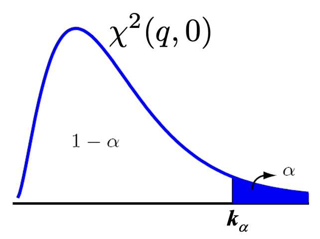
Fig. 3.16 PDF of \(\chi2\)(q,0)-distribution with threshold value \(k_{\alpha}\) based on chosen false alarm probability \(\alpha\).

This test is known as the Generalized Likelihood Ratio Test (GLRT). It can be derived by using the the ratio of the likelihood functions for \(\mathcal{H}_0\) and \(\mathcal{H}_a\) (recall that the BLUE solution is equal to the maximum likelihood solution in our case since the data are assumed to be normally distributed). This is a logical choice since the purpose of our test is to decide whether \(\mathcal{H}_0\) is sufficiently likely compared to \(\mathcal{H}_a\). The derivation is beyond the scope of MUDE.

Important to mention is that this is the most powerful test: no other test statistic can be found that would result in a larger detection power \(\gamma\) for the same \(\alpha\).

Exercise

Overall model test

Many options for the alternative hypothesis are possible, but instead of immediately testing the null hypothesis against a very specific alternative, it common to first apply the so-called overall model test (OMT): it is a test which just focuses on the validity of \(\mathcal{H}_0\) (how well do data and model fit) without having a specific \(\mathcal{H}_a\) in mind. This is identical to choosing the alternative hypothesis as follows:

\[\begin{split} \mathcal{H}_a:\;\; \mathbb{E}(\underset{m\times 1}{Y})=\underset{m\times m}{\begin{bmatrix} \underset{m\times n}{\mathrm{A}} & \underset{m\times m-n}{\mathrm{C}}\end{bmatrix}}\underset{m\times 1}{\begin{bmatrix}\mathrm{x}\\\nabla\end{bmatrix}} \end{split}\]

Hence, \(q=m-n\) and the matrix \(\begin{bmatrix}\mathrm{A} & \mathrm{C}\end{bmatrix}\) becomes a square invertible matrix, such that the system becomes determined and the BLUE follows as (try to show yourself):

\[\begin{split} \begin{bmatrix}\hat{X}_a \\ \hat{\nabla}\end{bmatrix} = \begin{bmatrix}\mathrm{A}&\mathrm{C}\end{bmatrix}^{-1}Y \end{split}\]

Answer

\[\begin{split} \begin{align*} \begin{bmatrix}\hat{X}_a \\ \hat{\nabla}\end{bmatrix} &= (\begin{bmatrix}\mathrm{A}&\mathrm{C}\end{bmatrix}^T\Sigma_Y^{-1} \begin{bmatrix}\mathrm{A}&\mathrm{C}\end{bmatrix})^{-1}\begin{bmatrix}\mathrm{A}&\mathrm{C}\end{bmatrix}^T\Sigma_Y^{-1}Y \\ &= \begin{bmatrix}\mathrm{A}&\mathrm{C}\end{bmatrix}^{-1}\Sigma_Y \begin{bmatrix}\mathrm{A}&\mathrm{C}\end{bmatrix}^{-T}\begin{bmatrix}\mathrm{A}&\mathrm{C}\end{bmatrix}^T\Sigma_Y^{-1}Y \\ &= \begin{bmatrix}\mathrm{A}&\mathrm{C}\end{bmatrix}^{-1}Y \end{align*} \end{split}\]

From this follows that the residuals become zero:

\[\begin{split} \hat{\epsilon}_a = Y- \begin{bmatrix}\mathrm{A}&\mathrm{C}\end{bmatrix}\begin{bmatrix}\hat{X}_a \\ \hat{\nabla}\end{bmatrix} = Y - \begin{bmatrix}\mathrm{A}&\mathrm{C}\end{bmatrix}\begin{bmatrix}\mathrm{A}&\mathrm{C}\end{bmatrix}^{-1}Y = 0 \end{split}\]

Hence, any alternative hypothesis for which the design matrix \(\begin{bmatrix}\mathrm{A}&\mathrm{C}\end{bmatrix}\) is an \(m\times m\) invertible matrix will result in residuals being equal to 0. This implies that any observed \(\mathrm{y}\) will satisfy the alternative hypothesis, which can thus also be formulated as

\[ \mathcal{H}_a:\;\; Y\in \mathbb{R}^m \]

The OMT is obtained from the GLRT:

\[ T_{q=m-n} = \hat{\epsilon}^T\Sigma_Y^{-1}\hat{\epsilon} > k_{\alpha} \]

since \(\hat{\epsilon}_a = 0\).

Exercise

Exercise

Estimation and testing procedure

If the OMT is accepted you are done and can present your estimation results, including precision and testing results. However, if the OMT is rejected, the next step would be to identify an alternative hypothesis that can be accepted. This might be an iterative procedure, since many options are possible for the alternative model.

The complete procedure is:

1. Define the nominal functional and stochastic model (under \(\mathcal{H}_0\))

2. Apply BLUE

3. Apply the overall model test (OMT)

4. If OMT accepted go to step 8; if OMT rejected go to step 5

5. Choose (another) specific alternative hypothesis

6. Apply generalized likelihood ratio test (GLRT) to decide whether the alternative hypothesis is indeed more likely

7. If alternative hypothesis accepted go to step 8; if rejected go back to step 5

8. Present estimates, precision and testing results

See the examples of common alternative hypotheses.

Outlier testing

Note that if you want to test for an outlier in an individual observation, there are in fact \(m\) alternative hypotheses to be considered. In that case, in step 6 we would apply the test for all \(m\) hypotheses and the one with the largest test statistic would be selected. However, it could be that there is more than one outlier. Therefore we would remove the outlying observation and go back to step 1. This procedure is repeated until no more outliers can be identified.

Exercise

Why would you select the alternative model with the largest test statistic?

Solution

The test statistic is given by \(T_q = \hat{\epsilon}^T\Sigma_Y^{-1}\hat{\epsilon}-\hat{\epsilon}_a^T\Sigma_Y^{-1}\hat{\epsilon}_a \). Hence,the alternative hypothesis with largest \(T_q\) must have the smallest weighted squared norm of residuals \(\hat{\epsilon}_a^T\Sigma_Y^{-1}\hat{\epsilon}_a \), and thus the best fit in a weighted least-squares sense.

Fig. 3.17 shows an example where on the left a linear trend is fitted to four observations without outliers. Here the overall model test would be accepted. On the right, the same example but with a bias of 10 mm added to the third observation. The bias has a large impact: the fitted line is pulled upwards with a much steeper slope. Consequently, the residuals of three observations become very large, which would result in a rejection of the overall model test. The green line shows the fitted model after removing the third observation.

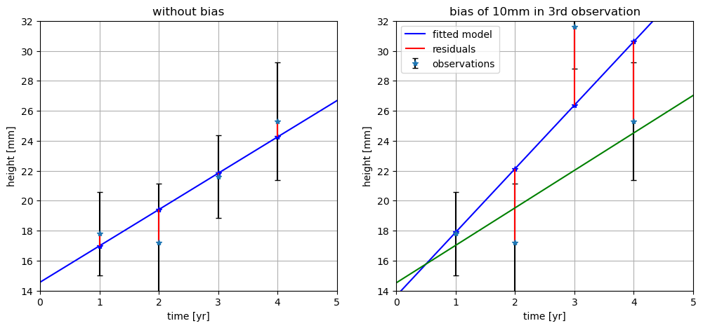
Fig. 3.17 Linear trend fitted to a set of four observations without (left) and with one outlier (right).

Model selection

In some cases, you may immediately want to test between two competing models, for instance if you are interested in the height change of a point over time you may want to test a linear trend model (constant velocity) versus a model including a constant acceleration. In that case, the procedure would be:

1. Define the functional and stochastic models (under \(\mathcal{H}_0\) and \(\mathcal{H}_a\))

2. Apply BLUE for both models

3. Apply the generalized likelihood ratio test (GLRT)

4. Present estimates, precision and testing results for accepted model

Attribution

This chapter was written by Sandra Verhagen. Find out more here.