6.1. Introduction and k-Nearest Neighbors

# pip install packages that are not in Pyodide
%pip install ipympl==0.9.3
%pip install seaborn==0.12.2

# Import the necessary libraries
import numpy as np
import matplotlib.pyplot as plt
from sklearn.neighbors import KNeighborsRegressor
from mude_tools import magicplotter
from cycler import cycler
import seaborn as sns

%matplotlib widget

# Set the color scheme
sns.set_theme()
colors = [
    "#0076C2",
    "#EC6842",
    "#A50034",
    "#009B77",
    "#FFB81C",
    "#E03C31",
    "#6CC24A",
    "#EF60A3",
    "#0C2340",
    "#00B8C8",
    "#6F1D77",
]
plt.rcParams["axes.prop_cycle"] = cycler(color=colors)

This page contains interactive python element: click –> Live Code in the top right corner to activate it.

Introduction

A very general problem often encountered is predicting some target variable \(t\) as a function of a predictor variable \(x\), but we only have inaccurate measurements of our target variable. Some examples of possible problems where we can apply this kind of framework are given below:

Problem	Target variable \(t\)	Predictor variable \(x\)
Structural health monitoring of a bridge	Displacement	Location along the bridge
Fatigue testing of a steel specimen	Stress	Number of loading cycles
Flood control of the river Maas	Volumetric flow rate	Precipitation in the Ardennes
Radioactive decay of a radon-222 sample	Number of \(\alpha\)-particles emitted	Time
Cooling rate of my coffee cup	Temperature	Time

To strip the problem down to its bare essentials, we will use a toy problem, where we actually know the ground truth \(f(x)\). In our case, this will be a simple sine wave, of which we make 100 noisy measurements from \(x=0\) to \(x=2 \pi\). Note that, in a practical setting, we would only have access to these noisy measurements and not to the true function that generated the data. Finding a good estimate of \(f(x)\) based on this contaminated data is one of our main objectives.

# The true function relating t to x
def f_truth(x, freq=1, **kwargs):
    # Return a sine with a frequency of freq
    return np.sin(x * freq)


# The data generation function
def f_data(epsilon=0.7, N=100, **kwargs):
    # Apply a seed if one is given
    if "seed" in kwargs:
        np.random.seed(kwargs["seed"])

    # Get the minimum and maximum
    xmin = kwargs.get("xmin", 0)
    xmax = kwargs.get("xmax", 2 * np.pi)

    # Generate N evenly spaced observation locations
    x = np.linspace(xmin, xmax, N)

    # Generate N noisy observations (1 at each location)
    t = f_truth(x, **kwargs) + np.random.normal(0, epsilon, N)

    # Return both the locations and the observations
    return x, t

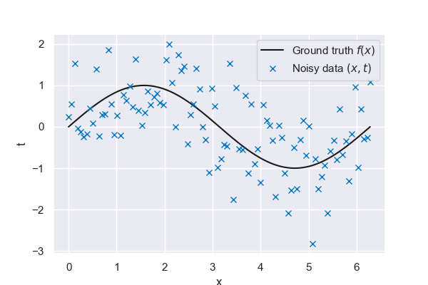
Fig. 6.24 100 noisy measurements from sine wave ground truth

k-nearest neighbors

A (perhaps naive) approach to find \(y(x)\) (i.e. the approximation of \(f(x)\)) would be to simply look at the surrounding data points and take their average to get an estimate of \(f(x)\). This approach is called k-nearest neighbors, where \(k\) refers to the number of surrounding points we are looking at.

Implementing this is not trivial, but thankfully we can leverage existing implementations. The KNeighborsRegressor function from the sklearn.neighbors library can be used to fit our data and get \(y(x)\) to make predictions.

# Define the prediction locations
# (note that these are different from the locations where we observed our data)
x_pred = np.linspace(0, 2 * np.pi, 1000)


# Define a function that makes a KNN prediction at the given locations, based on the given (x,t) data
def KNN(x, t, x_pred, k=1, **kwargs):
    # Convert x and x_pred to a column vector in order for KNeighborsRegresser to work
    X = x.reshape(-1, 1)
    X_pred = x_pred.reshape(-1, 1)

    # Train the KNN based on the given (x,t) data
    neigh = KNeighborsRegressor(k)
    neigh.fit(X, t)

    # Make a prediction at the locations given by x_pred
    y = neigh.predict(X_pred)

    # Check if the regressor itself should be returned
    if kwargs.get("return_regressor", False):
        # If so, return the fitted KNN regressor
        return neigh

    else:
        # If not, return the predicted values
        return y

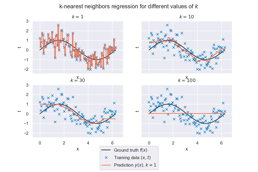
Fig. 6.25 k-nearest neighbors regression for different values of \(k\)

Looking at the previous plots, a few questions might pop up:

• For \(k=1\), we see that our prediction matches the observed data exactly in all data points. Is this desirable?

• For \(k=30\), what is going on around \(x=0\) and \(x=2 \pi\)?

• For \(k=100\), why is our prediction constant with respect to \(x\)?

Varying our model parameters

Clearly, some value of \(k\) between 1 and 100 would give us the best predictions. In the next interactive plot the following variables can be adjusted:

• \(N\), the size of the training data set

• \(\varepsilon\), the level of noise associated with the data

• \(k\), the number of neighbors over which the average is taken

• The seed can be updated to generate new random data sets

• The oscillation frequency of the underlying ground truth model, which controls how nonlinear the approximation should be

• A probing location \(x_0\), allowing you to see which neighbors are used to get the average response \(y(x_0)\) of the kNN estimator

plot1 = magicplotter(f_data, f_truth, KNN, x_pred)
plot1.fig.canvas.toolbar_visible = False
plot1.add_sliders("epsilon", "k", "N", "freq")
plot1.add_buttons("truth", "seed", "reset")
plot1.add_probe()
plot1.show()

Playing around with the plots

By visual inspection, use the slider of \(k\) to find its optimal value. The following questions might be interesting to ask yourself:

• If the training size \(N\) increases/decreases, how does this affect my optimal value of \(k\)?

Answer

In general, the more data we have, the more complex we can allow our model to be. But kNN estimators can be somewhat exceptional in this regard, here we tend to see higher values of \(k\) produce a visually better result for larger datasets.

• If the frequency increases/decreases, how does this affect my optimal value of \(k\)?

Answer

The frequency is related to how nonlinear our ground truth is. Excessive averaging (higher \(k\)) might be detrimental in this scenario. And of course, the more complex our process is, the more data we will need

• If my measurements are less/more noisy, how does this affect my optimal value of \(k\)?

Answer

Fitting noise is one of the main causes of overfitting. The less noise we have the lesser the risk of overfitting. Keep in mind however that even models trained on zero-noise datasets can overfit (i.e. give senseless predictions between data points). Reducing the noise here makes the resulting model less sensitive to our choice of \(k\).

• If I generate new data by changing the seed, how is my prediction affected for small values of \(k\)? What about large values of \(k\)?

Answer

This will become quite clear after watching all the videos for this week. Models with low \(k\) have high variance and low bias. High-variance models are highly sensitive to specific realizations of small datasets (this is why we say ‘high variance’). If these terms sound mysterious to you just keep going for now and come back after you have been through the whole content.

• So far, all observations were distributed uniformly over \(x\). How would our predictions change if our observed data was more clustered?

Answer

kNN regards on neighborhood data. You can have an idea of what would happen by looking at the edges of our sampling space (around \(x=0\) and \(x=6\)). Since there is nothing on the left (or right) of these points, kNN has to rely on a larger range of \(x\) values in order to be able to find the same number of neighbors. This degrades prediction performance quite a bit.

• If I do not know the truth, how do I figure out what my value of \(k\) should be?

Answer

In the next chapters we will go through concepts of model selection, including the definition of a validation dataset and how we can use it to make informed choices about model complexity.

Final remarks

So far, we have looked at our k-nearest neighbors regressor mostly qualitatively. However, it is possible to apply a more quantitative framework to our model and find the optimal value for \(k\) in a more structured way. The following video and accompanying chapter will discuss how this is done. See you there!

Attribution

This chapter is written by Iuri Rocha, Anne Poot, Joep Storm and Leon Riccius. Find out more here.