3.6. Maximum Likelihood Estimation

Maximum likelihood estimation is yet another estimation principle. In contrast to (weighted) least-squares and Best Linear Unbiased estimation, it relies on the probability distribution of the observables. Recall that for BLUE, we need to know the first two moments, given by the functional and stochastic model, respectively:

\[ \mathbb{E}(Y) = \mathrm{A} \mathrm{x}\;, \mathbb{D}(Y) = \Sigma_{Y}=\Sigma_{\epsilon} \]

in order to estimate the unknown parameters \(\mathrm{x}\). However, the solution \(\hat{X}\) does not depend on the underlying distribution of \(Y\).

Maximum likelihood principle

The principle of Maximum Likelihood estimation (MLE) is to find the most likely \(\mathrm{x}\) given a realization \(\mathrm{y}\) of \(Y\).

This boils down to estimating the unknown parameters \(\theta\) of the underlying distribution, which means that the probability density function (PDF) is known apart from the \(n\) parameters in \(\theta\). We will now distinguish between a PDF and likelihood function.

The probability density function \(f_Y(\mathrm{y}|\theta)\) is given as function of \(\mathrm{y}\) and with \(\theta\) known.

The likelihood function \(L(\theta|\mathrm{y})\) is given for a certain realization \(\mathrm{y}\) of \(Y\) as function of all possible values of \(\theta\).

With MLE, the goal is to find the \(\theta\) which maximizes the likelihood function for the given realization \(\mathrm{y}\).

Example exponential distribution

If \(Y\sim \text{Exp}(\lambda)\), the goal would be to estimate \(\lambda\) based on a realization \(\mathrm{y_{obs}}\) of \(Y\). Fig. 3.9 shows the PDF of \(Y\)

\[ f_Y(\mathrm{y}|\lambda)=\lambda \exp(-\lambda \mathrm{y}) \]

for different values of \(\lambda\). The likelihood function for the given \(\mathrm{y_{obs}}\) is shown on the right-hand side. It is shown that for instance the likelihood value for \(\lambda_1\) is equal to the corresponding density value in the left panel. The maximum likelihood estimate \(\hat{\lambda}\) is the value for which the likelihood function is maximized, in this case \(\hat{\lambda}=\lambda_2\), as shown in the figure.

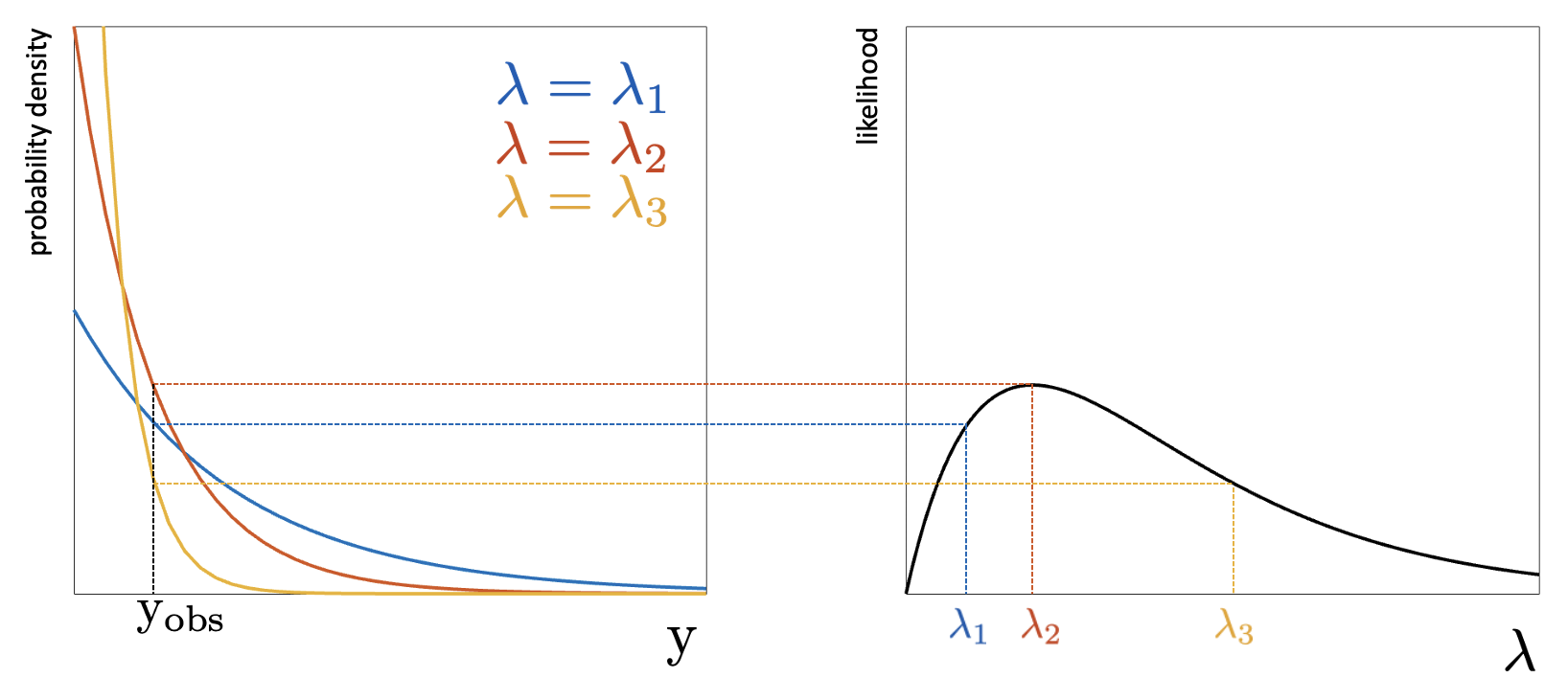
Fig. 3.9 PDF and likelihood function for exponential distribution.

Maximum Likelihood estimator of \(\mathrm{x}\)

We have that our observables are assumed to be normally distributed: \(Y\sim N(\mathrm{Ax},\Sigma_Y)\), where \(\mathrm{x}\) is unknown. The covariance matrix \(\Sigma_Y\) is assumed to be known, for instance from a calibration campaign.

Note

It is also possible to consider the case that \(\Sigma_Y\) is not (completely) known, for instance in case of a new sensor. Maximum Likelihood estimation can then also be applied to estimate this covariance matrix. However, this is beyond the scope of MUDE.

The likelihood function of the multivariate normal distribution is given by:

\[ L(\mathrm{Ax},\Sigma_Y|\mathrm{y})=\underset{c}{\underbrace{(\det{2\pi \Sigma_Y})^{-0.5}}}\exp\left(-\frac{1}{2}\mathrm{(y-Ax)^T} \Sigma_Y^{-1}(\mathrm{y-Ax})\right) \]

Maximizing this likelihood function for \(\mathrm{x}\) means that we have to find the \(\mathrm{x}\) such that:

• the first-order partial derivatives (gradient) are zero: \(\partial_{\mathrm{x} }L(\mathrm{Ax},\Sigma_Y|\mathrm{y})=0\)

• the second-order partial derivatives are negative.

Instead of working with the likelihood function, we prefer to work with the loglikelihood function:

\[ \ln L(\mathrm{Ax},\Sigma_Y|\mathrm{y})=\ln c -\frac{1}{2}\mathrm{(y-Ax)^T} \Sigma_Y^{-1}(\mathrm{y-Ax}) \]

since that is easier and results in the same maximum. Setting the gradient to zero gives:

\[\begin{split} \begin{align*} \frac{\partial \ln L(\mathrm{Ax},\Sigma_Y|\mathrm{y})}{\partial \mathrm{x}}&= \frac{\partial (-\frac{1}{2}\mathrm{(y-Ax)^T} \Sigma_Y^{-1}(\mathrm{y-Ax}))}{\partial \mathrm{x}}\\ &= -\frac{1}{2}(-2\mathrm{A^T} \Sigma_Y^{-1} Y+2\mathrm{A^T} \Sigma_Y^{-1} \mathrm{A}\mathrm{x})=0\\ \mathrm{A^T} \Sigma_Y^{-1} \mathrm{A}\mathrm{x} &= \mathrm{A^T} \Sigma_Y^{-1} \mathrm{y} \end{align*} \end{split}\]

The maximum likelihood estimate for a given realization \(\mathrm{y}\) follows thus as:

\[ \hat{\mathrm{x}}= (\mathrm{A^T} \Sigma_Y^{-1} \mathrm{A})^{-1} \mathrm{A^T} \Sigma_Y^{-1} \mathrm{y} \]

It can be verified that the second-order partial derivatives are \(-\mathrm{A^T} \Sigma_Y^{-1} \mathrm{A}\) and hence indeed negative (since \(\mathrm{A^T} \Sigma_Y^{-1} \mathrm{A}\) is positive definite).

MUDE exam information

You will not be asked to derive the MLE solution as above.

If we now replace the realization \(\mathrm{y}\) by the random observable vector \(Y\) we obtain the Maximum Likelihood estimator of \(\mathrm{x}\):

\[ \hat{X}= (\mathrm{A^T} \Sigma_Y^{-1} \mathrm{A})^{-1} \mathrm{A^T} \Sigma_Y^{-1} Y \]

It follows that the Maximum Likelihood estimator of \(\mathrm{x}\) is identical to the BLUE if \(Y\) is normally distributed.

Attribution

This chapter was written by Sandra Verhagen. Find out more here.