5.1. PDF and CDF#
Probability Density Function (PDF)#
To mathematically describe the distribution of probability for a continuous random variable, we define the probability density function (PDF) of \(X\) as \(f_X(x)\), such that
To qualify as a probability distribution, the function must satisfy the conditions \(f_X(x) \geq 0\) and \(\int_{-\infty}^{+\infty}f_X(x)dx =1\), which can be related to the axioms. Note that in this case we use lower case \(x\) as the argument of the PDF, and upper case \(X\) denotes the random variable. Similarly, the function \(f_Y(u)\) describes the PDF of the random variable \(Y\). For notational convenience we will omit the subscript in the remainder of this chapter.
Cumulative Distribution Function (CDF)#
It’s important to realize that while the PDF describes the distribution of probability across all values of the random variable, probability density is not equivalent to probability. The density allows us to quantify the probability of a certain interval of the continuous random variable, through integration. In the equation below, the mathematical relationship between the CDF (denoted here as \(F(x)\)) and the PDF (denoted as \(f(x)\)) is shown.
The definition of the CDF includes an integral that begins at negative infinity and continues to a specific value, \(x\), which defines the interval over which the probability is computing. In other words, the CDF gives the probability that the random variable \(X\) has a value less than \(x\).
Below, you find an interactive element that illustrates the relationship between the integral of the pdf and the cdf value. They grey-shaded area in the left subplot corresponds to the integral from \(-\infty\) to \(x\). Move your mouse over either the subplots and try to develop an intuition for how both distributions relate to each other. When is the cdf steep, when is it flat?
Fig. 5.1 Interactively visualize the relationship between the PDF and the CDF (the integral of the PDF value).#
It should be easy to see from the definition of the CDF that the probability of observing an exact value of a continuous random variable is exactly zero. This is an important observation, and also an important characteristic that separates continuous and discrete random variables.
PDF and CDF of Gaussian distribution#
You have already extensively used one parametric distribution! Does it ring the bell ‘the bell curve’? During your BSc, you have probably used the Normal or Gaussian distribution, whose PDF presents a bell shape. The PDF of the Normal distribution is given by
where \(x\) is the value of the random variable and \(\mu\) and \(\sigma\) are the two parameters of the distribution. Thus, you can see that through the previous equation we establish a relationship between the probability densities and the values of the random variable. In the case of the Normal distribution, the parameters \(\mu\) and \(\sigma\) correspond to the mean and standard deviation of the random variable. However, this is not the case for all the distributions and it is also dependent on how it is parameterized.
As you have already seen, the previous expression provides us with probability densities, so we need to integrate it to obtain actual probabilities through the CDF (non-exceedance probabilities). In the case of the Normal distribution, there is no closed form of the CDF (the integral).
Let’s see how the distribution looks. In the figure below, the PDF and CDF of the Gaussian distribution are shown for different values of its parameters. In the PDF plot, you can see the bell shape that was already mentioned. You will learn more about how this distribution behaves later on.
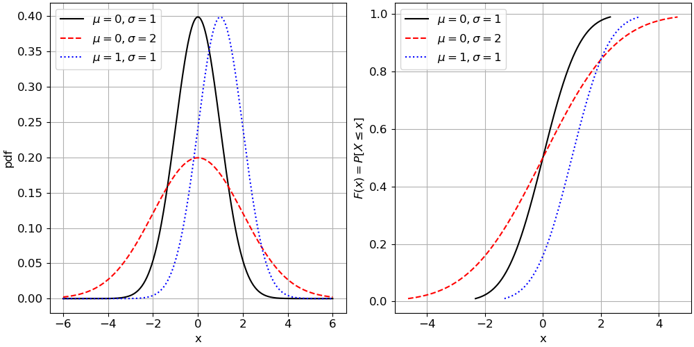
Fig. 5.2 Gaussian distribution function: PDF and CDF.#
Below, you will find an interactive element that allows you to explore the influence of different means and standard deviations on the PDF and CDF. Experiment with both options and observe how it affects the shape of both distributions.
Fig. 5.3 Interactively change the mean and standard deviation of the Gaussian distribution to visualize the effect on the PDF and CDF.#
Probability of other intervals#
We saw that the CDF provides us with the non-exceedance probabilities, this is \([-\infty, x]\). But what happens if we are interested in the probabilities of another intervals? It is common to be interested in the probability of exceeding a value. For instance, wind speeds over a value can damage an structure or concentrations of a nutrient higher than a value can lead to eutrophication. Therefore, we want to integrate from a value \(x\) to \(\infty\). Here the probability axioms make this easy, since the PDF integrates to 1 over the sample space of the random variable:
The figure below shows both the CDF and the complementary CDF.
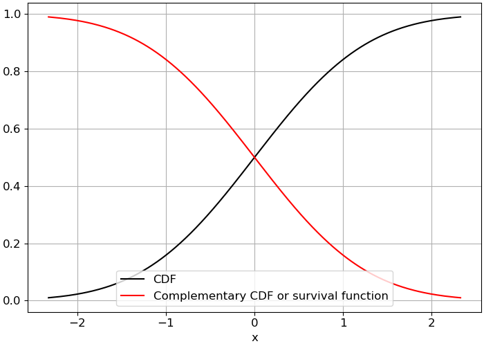
Fig. 5.4 Gaussian distribution function: CDF and survival function or complemetary CDF.#
Thus, the exceedance probabilities can be directly computed by substracting to 1 the non-exceedance probabilities obtained from the CDF. The result is called the complementary CDF. However, this function has many alternative names. The name survival function may sound odd due to its positive connotation, but this is appropriate when the random variable describes, for example, the lifetime of a structure.
Another interval is that between two values, \(x_1\) and \(x_2\) (where \(x_2>x_1\)). Using the CDF, \(F(x_2)\), gives the probability of values below \(x_2\) but also those below \(x_1\). Then, we need to substract \(F(x_2)-F(x_1)\) to obtain the probability of being in the interval \([x_1, x_2]\). In mathematical terms:
Inverse CDF#
Often, in regulations and guidelines, it is required to design our structure or system for a value which is not exceeded more than \(p\) percent of the time. Thus, we are facing the opposite problem: what is the value of the random variable, \(x\), whose non-exceedance probability has a specified value, \(p\)? The solution is simple: the inverse of the CDF, \(x = F^{-1}(p)\). As previously mentioned, the CDF is just an equation which in most occasions can be solved analytically, so we just need to work through the formula and calculate \(x\) given \(p\).
Attribution
This chapter was written by Patricia Mares Nasarre and Robert Lanzafame. Find out more here.