3.8. Model testing

In Chapter Precision and confidence intervals one part of the quality assessment was presented. But evaluating the precision does not tell us how well the model fits the data we collected. It might be that we worked with a wrong functional model (e.g., too simplistic), or a wrong stochastic model. Or it may be that our observations are affected by blunders or systematic biases.

In some cases, a first indication that something may be wrong can be obtained by plotting the observations and the fitted model together with the confidence intervals. If the residuals are large compared to the confidence interval this is obviously an indication that something is wrong. Another indication is if you see a clear pattern in the residuals once you plot those as function of time or location.

Example volcano deformation

For the volcano deforomation example, the observed and modelled deformations are shown in Fig. 3.12, as well as the residuals (on the right). In this case, we can see some ‘patterns’: two clusters with positive residuals in the upper-left and lower-right corner, where an uplift is observed which is not accounted for by the model. There is also a cluster of negative residuals, where the subsidence is larger than the model predicts. The model assumed a spherical deformation, which is apparently too simplistic.

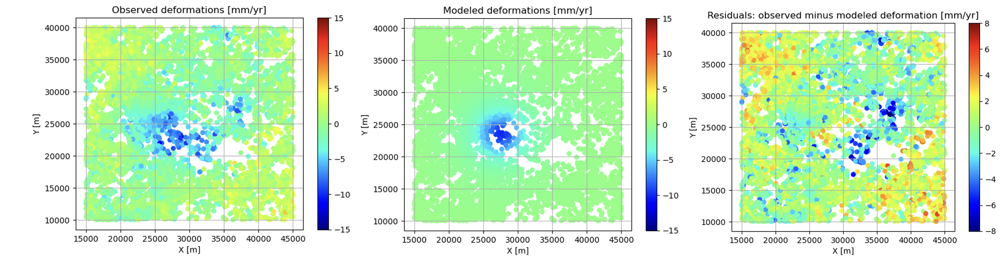
Fig. 3.12 Observed deformation rates above a magma chamber (left), the modelled deformation after applying non-linear least-squares (middle), and the residuals (right).

However, it is not always straightforward to decide whether the residuals are too large or show a suspicious pattern, especially for models with more than two unknown parameters. Moreover, the question remains: is the fit good enough or not? And if not, what is the underlying misspecification/error?

To answer these questions, we need to apply statistical hypothesis testing. In this chapter, we will introduce the hypothesis testing principle, and then explain how it can be applied in sensing and monitoring to:

• test for blunders or systematic biases in the observations;

• test for misspecifications of the functional model and/or decide between two competing hypotheses regarding the functional model.

Statistical hypothesis testing: principle

Statistical hypothesis testing means that we apply a certain test to decide between two (or more) competing hypothesis regarding the underlying model (in our case the functional or stochastic model). Therefore we assume a nominal model, corresponding to the null hypothesis \(\mathcal{H}_0\), and another model for the alternative hypothesis \(\mathcal{H}_a\).

An important note to be made here is that the null hypothesis is presumed to be true unless the data provides convincing evidence against it (i.e., there is significant misfit).

This is similar as in the court house: a defendant is presumed to be innocent until proven guilty based on convincing evidence.

Example laser distometer

We would like to test whether a laser distometer is well-calibrated, implying that the mean error of repeated measurements should be zero (null hypothesis). An alternative hypothesis in this case could be that all measurements are affected by a certain constant offset (i.e., systematic bias). We can also write this as:

\[\begin{split} \begin{align*} \mathcal{H}_0: \mathbb{E}(\epsilon) &= 0 \\ \mathcal{H}_a: \mathbb{E}(\epsilon) &= \nabla \end{align*} \end{split}\]

The next step is then to define a so-called test statistic \(T\) with a known distribution. Based on the actual observations, a realization of this test statistic can be computed and it can be assessed whether this realization is a likely outcome given the distribution. This can be illustrated based on the example.

Example laser distometer (continued)

Assuming that the random errors of the observed distances with the laser distometer are normally distributed with zero mean and standard deviation \(\sigma\), a logical choice for the test statistic would be simply to use the mean error. To test whether the laser distometer is well-calibrated we measure a known distance \(d\) \(m\) times, such that we can calculate the errors \(\epsilon_i = y_i - d\) (\(i=1,\ldots,m\)). All measurements are assumed to be independent. Applying the variance propagation law, we find that the variance of the mean error will be \(\frac{\sigma^2}{m}\).

We thus have for the null and alternative hypothesis:

\[\begin{split} \begin{align*} \mathcal{H}_0: T= \frac{1}{m}\sum_{i=1}^{m} \epsilon_i \sim N(0,\frac{\sigma^2}{m}) \\ \mathcal{H}_a: T= \frac{1}{m}\sum_{i=1}^{m} \epsilon_i \sim N(\nabla ,\frac{\sigma^2}{m}) \end{align*} \end{split}\]

Fig. 3.13 shows the PDFs of the test statistic under the null and alternative hypothesis. Based on the distributions, the null hypothesis is obviously more likely in case the observed mean error (realization of \(T\)) is smaller than \(k\). Therefore the null hypothesis would be accepted if \(T \leq k\) and rejected otherwise. The corresponding acceptance and critical region are also shown.

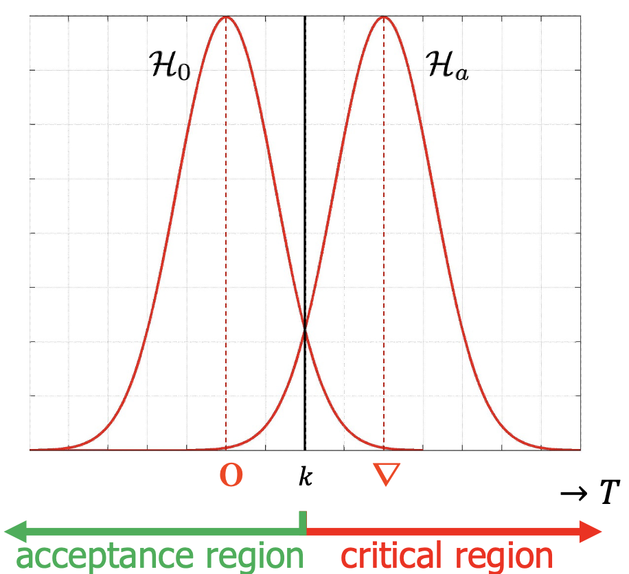
Fig. 3.13 PDFs of test statistic \(T\) under null and alternative hypothesis, with threshold value \(k\).

Even though the choice for the threshold value in the example above may seem logical, it does not account for the requirement that there should be convincing evidence against the null hypothesis being true. Even though the probability that the test statistic is larger than \(k\) if the null hypothesis is true, \(P(T>k | \mathcal{H}_0)\), is small, it is not zero! A better approach would therefore be to determine the threshold value based on the choice of an acceptable false alarm probability \(\alpha\), since a false alarm (also referred to as type I error) corresponds to rejecting the null hypothesis while it is true.

Definition

The false alarm or type I error probability \(\alpha\) is defined as:

\[ \alpha = P(T \in \mathcal{C}|\mathcal{H}_0) \]

where \(\mathcal{C}\) is the critical region.

In the example, the bias was assumed to be positive, such that there is a right-side critical region \(\mathcal{C}\), but in practice the bias may also be negative (left-side critical region), or we may have a two-sided critical region.

See Fig. 3.14, where the principle has been applied for the same example as above. Given that under the null hypothesis \(T\sim N(0,\sigma^2/m)\), we can easily determine the threshold value \(k_{\alpha}\) for a given \(\alpha\) using the inverse CDF. The critical region \(\mathcal{C}\) is thus given by \(T>k_{\alpha}\).

Fig. 3.14 PDFs of test statistic \(T\) under null and alternative hypothesis, with false alarm probability \(\alpha\) and threshold value \(k_{\alpha}\).

Besides the probability of a false alarm, the figure also shows the probability of false acceptance of \(\mathcal{H}_0\), referred to as the type II error probability, or missed detection probability. In this case, the alternative hypothesis is true, but still the null hypothesis is accepted.

Definitions

The missed detecion or type II error probability \(\beta\) is defined as:

\[ \beta= P(T\notin \mathcal{C}|\mathcal{H}_a) \]

where \(\mathcal{C}\) is the critical region.

The detection power or probability of detection is:

\[ \gamma = 1-\beta \]

Ideally, both the type I and type II error probabilities should be small. However, as can be seen from the figure, choosing a smaller value for \(\alpha\) implies a larger \(\beta\) and vice versa.

The decision matrix in decision summarizes the four types of decisions and corresponding probabilities.

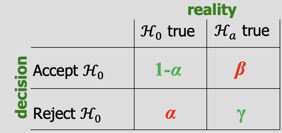
Fig. 3.15 Decision matrix for hypothesis testing.

Exercise

Attribution

This chapter was written by Sandra Verhagen. Find out more here.