5. Uncertainty Propagation#
Attribution
This chapter was written by Sandra Verhagen and Lotfi Massarweh. Find out more here.
Most quantities we estimate in engineering and sciences are functions of uncertain inputs. For a given stochastic input \(Y\) and a generic transformation \(q: \mathbb{R} \rightarrow \mathbb{R}\), also the output \(X = q(Y)\) is expected to be random. However, if we know the distribution of the input data \(Y\), it is in general non-trivial to fully define the distribution of the output data \(X\) (see Fig. 5.1). The propagation of the uncertainty allows us to indeed acquire information on the transformed distribution, nonetheless this is not always simple and some approximations might be needed.
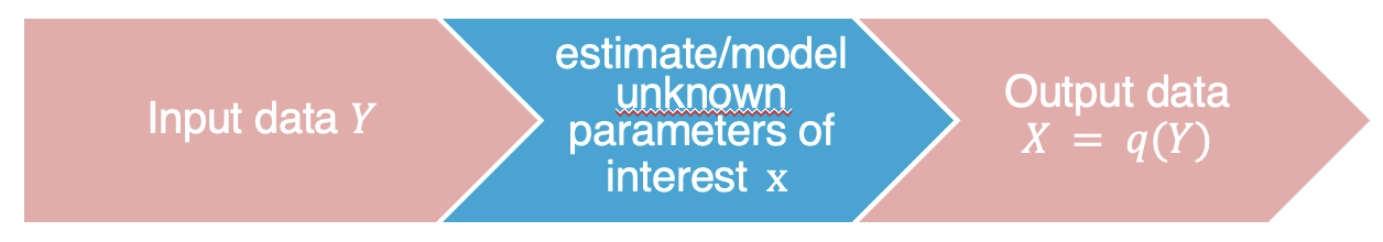
Fig. 5.1 Given a random input \(Y\), the model output \(X\) is also expected to be random.#
Some simple examples of functions are that may have uncertain inputs are:
Temperature conversion from Celsius to Fahrenheit
\(T_f = q(T_c) = \frac{9}{5} T_c + 32\)
Compute the mean of \(m\) repeated measurements \(Y_i\)
\(\hat{X} = q(Y_1,\ldots,Y_m)=\frac{1}{m}\sum_{i=1}^m Y_i\)
Subsurface temperature \(T_z\) as a function of depth \(Z\) and surface temperature \(T_0\), given a known factor \(a\)
\(T_z = q(T_0,Z) = T_0 + a \cdot Z\)
Wind loading \(F\) on a building as function of area of building face \(A\), wind pressure \(P\), drag coefficient \(C\)
\(F = q(A,P,C) = A \cdot P \cdot C\)
Evaporation \(Q\) using Bowen Ratio Energy Balance as function of the net radiation \(R\), ground heat flux \(G\), bowen ratio \(B\)
\(Q = q(R,G,B) = \frac{R-G}{1-B}\)
You can think of scenarios where inputs of these functions follow a known distribution. In this chapter we explore what can then be said about the resulting uncertainty on the outputs.
The main question we are interested in is:
How does the statistical uncertainty in the input data propagate into the output variables?
In this chapter, we will try to answer this question and we will focus on propagating and combining the uncertainty through functions of random variables. This is fundamental since functions of random variables naturally occur when solving real-world problems.
We will start by describing how to transform random variables, and make an illustrative example. Then, we will consider propagating the first two moments, namely the mean (or expectation) and the variance (or dispersion). This will be considered for transformations based on linear and linearized functions of the input. Lastly, when analytical solutions or approximations are no easy to be found, we will show how Monte Carlo simulation methods could be adopted for the uncertainty propagation.