3.7. Non-linear least-squares estimation

Let the non-linear system of observation equations be given by:

\[\begin{split} \mathbb{E} ( \begin{bmatrix} Y_1\\ Y_2\\ \vdots\\ Y_m \end{bmatrix} ) = q(\mathrm{x}) = \begin{bmatrix} q_{1}(\mathrm{x})\\ q_{2}(\mathrm{x})\\ \vdots\\ q_{m}(\mathrm{x}) \end{bmatrix} \end{split}\]

This system cannot be directly solved using the weighted least-squares or the best linear unbiased estimators. Here, we will introduce the non-linear least-squares principle, based on a linearization of the system of equations.

One example of a non-linear problem is the positioning model.

Example volcano deformation

Observable \(Y_i\) is deformation rate at known location \((x_i,y_i)\) due to an unknown volume change \(\Delta V\) of a magma chamber at unknown depth \(d\). The observation equation according to the so-called Mogi model would be:

\[ \mathbb{E} ( Y_i)=q_i(\Delta V, d, x_s, y_s)=\frac{0.73\Delta V}{\pi d^2} \left(1 + \frac{1}{d^2}\left((x_i − x_s)^2 + (y_i − y_s)^2\right)\right)^{-3/2} \]

where \((x_s,y_s)\) are the unknown horizontal coordinates of the centre of the magma chamber. This observation equation is non-linear in three out of the four unknowns.

Fig. 3.10 shows a spatial dataset with 10,000 observed deformation rates above a magma chamber. Hence we have a system of 10,000 non-linear observation equations in four unknowns. How to solve it?

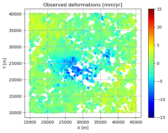
Fig. 3.10 Observed deformation rates above a magma chamber.

Video

Linearization

For the linearization we need the first-order Taylor polynomial, which gives the linear approximation of for instance the first observable \(Y_1 = q_1(\mathrm{x})\) at \(\mathrm{x}=\mathrm{x}_{[0]}\) as:

\[ Y_1\approx q_1( \mathrm{x}_{[0]})+ \partial_{x_1} q_1(\mathrm{x}_{[0]})\Delta \mathrm{x}_{[0]}+ \partial_{x_2} q_1(\mathrm{x}_{[0]})\Delta \mathrm{x}_{[0]}+ \ldots + \partial_{x_n} q_1(\mathrm{x}_{[0]})\Delta \mathrm{x}_{[0]} \]

where \(\Delta \mathrm{x}_{[0]} = \mathrm{x}- \mathrm{x}_{[0]}\) and \(\mathrm{x}_{[0]}\) is the initial guess of \(\mathrm{x}\). Note that for now we ignore the random errors in the equations.

Let us now consider the difference between the observable \(Y_1\) and the solution of the forward model at \(\mathrm{x}_{[0]}\):

\[\begin{split} \begin{align*} \Delta Y_{1[0]} &= Y_1- q_1(\mathrm{x}_{[0]}) \\ &\approx \left[ \partial_{x_1} q_1(\mathrm{x}_{[0]}) \quad \partial_{x_2} q_1(\mathrm{x}_{[0]}) \quad \ldots \quad \partial_{x_n} q_1(\mathrm{x}_{[0]})\right]\Delta \mathrm{x}_{[0]} \end{align*} \end{split}\]

which we refer to as the observed-minus-computed observable. Note that \(\Delta \mathrm{x}_{[0]}\) is an \(n\times 1\) vector.

We can now obtain the linearized functional model:

\[\begin{split} \begin{align*} E\{\begin{bmatrix} \Delta Y_1 \\ \Delta Y_2 \\ \vdots \\ \Delta Y_m \end{bmatrix}_{[0]}\} &=\begin{bmatrix} \partial_{x_1} q_1(\mathrm{x}_{[0]}) &\partial_{x_2} q_1(\mathrm{x}_{[0]}) & \ldots & \partial_{x_n} q_1(\mathrm{x}_{[0]}) \\ \partial_{x_1} q_2(\mathrm{x}_{[0]}) &\partial_{x_2} q_2(\mathrm{x}_{[0]}) & \ldots & \partial_{x_n} q_2(\mathrm{x}_{[0]}) \\ \vdots & \vdots & \ddots & \vdots\\ \partial_{x_1} q_m(\mathrm{x}_{[0]}) &\partial_{x_2} q_m(\mathrm{x}_{[0]}) & \ldots& \partial_{x_n} q_m(\mathrm{x}_{[0]}) \end{bmatrix}\Delta \mathrm{x}_{[0]} \\ &= \mathrm{J}_{[0]}\Delta \mathrm{x}_{[0]}\end{align*} \end{split}\]

with Jacobian matrix \(\mathrm{J}_{[0]}\).

And this allows to apply best linear unbiased estimation (BLUE) to get an estimator for \(\Delta \mathrm{x}_{[0]}\):

\[ \Delta \hat{X}_{[0]}=\left(\mathrm{J}_{[0]}^T \Sigma_{Y}^{-1} \mathrm{J}_{[0]} \right)^{-1}\mathrm{J}_{[0]}^T \Sigma_{Y}^{-1}\Delta Y_{[0]} \]

since the Jacobian \( \mathrm{J}_{[0]}\) takes the role of the design matrix \(\mathrm{A}\) and the observation vector is replaced by its \(\Delta\)-version as compared to the BLUE of the linear model \(\mathbb{E}(Y) = \mathrm{Ax}\).

Since we have \(\Delta \mathrm{x}_{[0]} = \mathrm{x}- \mathrm{x}_{[0]}\), an “estimator” of \(\mathrm{x}\) can thus be obtained as:

\[ \hat{X}=\mathrm{x}_{[0]}+\Delta \hat{X}_{[0]} \]

However, the quality of the linear approximation depends very much on the closeness of \(\mathrm{x}_{[0]}\) to \(\mathrm{x}\). Therefore, instead we apply an iterative procedure, which means that we repeat the process with \(\mathrm{x}_{[1]}=\mathrm{x}_{[0]}+\Delta \hat{X}_{[0]}\) as our new guess. This procedure is continued until the \(\Delta \hat{\mathrm{x}}_{[i]}\) becomes small enough. This is called the Gauss-Newton iteration procedure, and is shown in the scheme below.

Gauss-Newton iteration

See Fig. 3.11 for an illustration of the iterative procedure, referred to as the Gauss-Newton iteration.

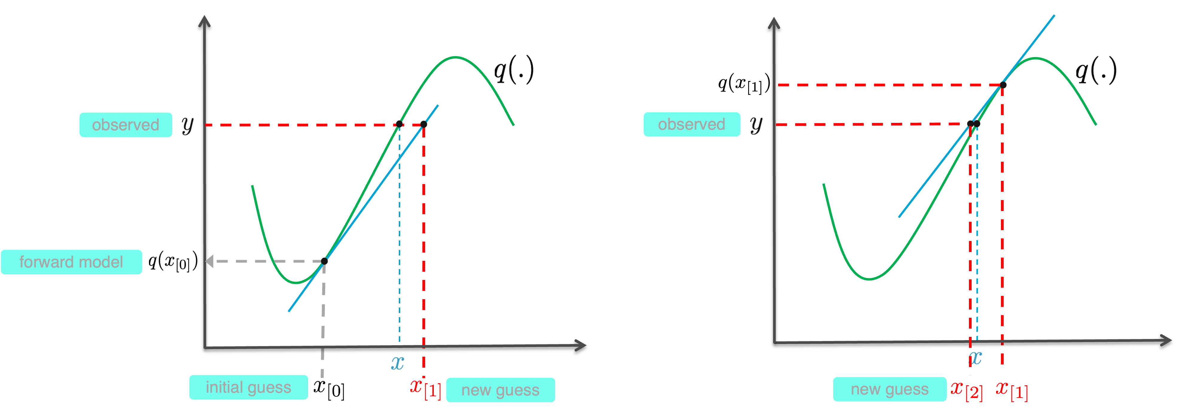
Fig. 3.11 Visualization of two iteration steps of Gauss-Newton iteration. The non-linear function \(q\) is shown, together with the linear approximations (blue line) at \(q(x_{[i]})\) in each step.

Assume we have the observation vector \(\mathrm{y}\) (realization of \(Y\)).

Start with initial guess \(\mathrm{x}_{[0]}\), and start iteration with \(i=0\)

1. Calculate observed-minus-computed \(\Delta \mathrm{y}_{[i]} = \mathrm{y} - q(\mathrm{x}_{[i]}) \)

2. Determine the Jacobian \(\mathrm{J}_{[i]}\)

3. Estimate \(\Delta \hat{\mathrm{x}}_{[i]}=\left(\mathrm{J}_{[i]}^T \Sigma_{Y}^{-1} \mathrm{J}_{[i]} \right)^{-1}\mathrm{J}_{[i]}^T \Sigma_{Y}^{-1}\Delta \mathrm{y}_{[i]}\)

4. New guess \(\mathrm{x}_{[i+1]}=\Delta\hat{\mathrm{x}}_{[i]}+ \mathrm{x}_{[i]}\)

5. If stop criterion is met: set \(\hat{\mathrm{x}}=\mathrm{x}_{[i+1]}\) and break, otherwise set \(i:=i+1\) and go to step 1

In this scheme we need to choose a stop criterion, for which we use:

\[ \Delta \hat{\mathrm{x}}_{[i]}^T \mathrm{N}_{[i]} \Delta \hat{\mathrm{x}}_{[i]} < \delta \;\; \text{with} \;\;\mathrm{N}_{[i]}=\mathrm{J}_{[i]}^T \Sigma_{Y}^{-1} \mathrm{J}_{[i]} \]

The normal matrix \(\mathrm{N}_{[i]}\) is used as a weight matrix, since it is equal to the inverse of the covariance matrix of the estimated \(\Delta \hat{\mathrm{x}}_{[i]}\), and estimated parameters with small variance should have a relatively small deviation compared to parameters with large variance.

The threshold \(\delta\) must be set to a very small value, e.g., \(10^{-8}\).

Once the stop criterion is met, we say that the solution converged, and the last solution \( \mathrm{x}_{[i+1]}\) is then finally used as our estimate of \(\mathrm{x}\).

Exercise

Remarks and properties

There is no default recipe for making the initial guess \(\mathrm{x}_{[0]}\); it must be made based on insight into the problem at hand. A good initial guess is important for two reasons:

• a bad initial guess may result in the solution NOT to converge;

• a good initial guess will speed up the convergence, i.e. requiring fewer iterations.

The covariance matrix of \(\hat{X}\) is given by:

\[ \Sigma_{\hat{X}}=\left(\mathrm{J}_{[i]}^T \Sigma_{Y}^{-1} \mathrm{J}_{[i]} \right)^{-1} \]

although this is not strictly true. The estimator \(\hat X\) is namely NOT a best linear unbiased estimator of \(\mathrm{x}\) since we used a linear approximation. And since the estimator is not a linear estimator due to ignoring the higher-order terms, it is not normally distributed.

However, in practice the linear (first-order Taylor) approximation often works so well that the performance is very close to that of BLUE and we may assume the normal distribution.

As a final note we would like to mention that the Gauss-Newton method is just one approach for solving a non-linear least-squares problem. In practice, especially for highly non-linear problems, the Levenberg-Marquardt method is often used. It can be considered as a refinement of the Gauss-Newton method with a higher chance of convergence.

Attribution

This chapter was written by Sandra Verhagen. Find out more here.