Glacier Melting Model#
You have 12 monthly measurements of the height of a point on a glacier. The measurements are obtained from a satellite laser altimeter. The observations are given in the code below.
We will fit a model assuming a linear trend (constant velocity) to account for the melting, plus an annual signal due to the seasonal impact on ice. Formulating a generalized form of this model is part of your task below. Note, however, that the periodic signal can be implemented in many ways. For this assignment you can assume that the periodic term is implemented as follows:
where \(\phi\) is the phase angle, which we will assume is 0 for this workshop and will leave out of the model formulation in order to keep our model linear (i.e., leave it out of the A-matrix).
The precision (1 \(\sigma\)) of the first six observations is 0.7 meter, the last six observations have a precision of 2 meter due to a change in the settings of the instrument. All observations are mutually independent.
import numpy as np
from scipy.stats import norm
import matplotlib.pyplot as plt

# this will print all float arrays with 3 decimal places
float_formatter = "{:.3f}".format
np.set_printoptions(formatter={'float_kind':float_formatter})
Part 1: Observation model#
First we will construct the observation model, based on the following information that is provided: times of observations, observed heights and number of observations.
Task 1.1:
Complete the definition of the observation time array times and define the other variables such that the print statements correctly describe the design matrix A.
Use times=0 as the first point.
y = [59.82, 57.20, 59.09, 59.49, 59.68, 59.34, 60.95, 59.34, 55.38, 54.33, 48.71, 48.47]

times = np.arange(12)
number_of_observations = len(times)
number_of_parameters = 3

print(f'Dimensions of the design matrix A:')
print(f'  {number_of_observations:3d} rows')
print(f'  {number_of_parameters:3d} columns')
Dimensions of the design matrix A:
   12 rows
    3 columns
Next, we need to assemble the design matrix in Python. Rather than enter each value manually, we have a few tricks to make this easier. Here is an example Python cell that illustrates how one-dimensional arrays (i.e., columns or rows) can be assembled into a matrix in two ways:
As diagonal elements, and
As parallel elements (columns, in this case)
Note also the use of np.ones() to quickly make a row or column of any size with the same values in each element.
column_1 = np.array([33333, 0, 0])
column_2 = 99999*np.ones(3)

example_1 = np.diagflat([column_1, column_2])
example_2 = np.column_stack((column_1, column_2))

print(example_1, '\n\n', example_2)
[[33333.     0.     0.     0.     0.     0.]
 [    0.     0.     0.     0.     0.     0.]
 [    0.     0.     0.     0.     0.     0.]
 [    0.     0.     0. 99999.     0.     0.]
 [    0.     0.     0.     0. 99999.     0.]
 [    0.     0.     0.     0.     0. 99999.]]

 [[33333. 99999.]
 [    0. 99999.]
 [    0. 99999.]]
See documentation on np.diagflat and np.column_stack if you would like to understand more about these Numpy methods.
Task 1.2:
Complete the \(\mathrm{A}\)-matrix (design matrix) and covariance matrix \(\Sigma_Y\) (stochastic model) as a linear trend with an annual signal. The assert statement is used to confirm that the dimensions of your design matrix are correct (an error will occur if not).
A = np.column_stack((np.ones(number_of_observations),
                     times,
                     np.cos(2*np.pi*times/12)))
diag_1 = 0.7**2 * np.ones((1,6))
diag_2 = 2**2 * np.ones((1,6))
Sigma_Y = np.diagflat([diag_1,
                       diag_2])

assert A.shape == (number_of_observations, number_of_parameters)
2. Least-squares and Best linear unbiased (BLU) estimation#
The BLU estimator is a linear and unbiased estimator, which provides the best precision, where:
linear estimation: \(\hat{X}\) is a linear function of the observables \(Y\),
unbiased estimation: \(\mathbb{E}(\hat{X})=\mathrm{x}\),
best precision: sum of variances, \(\sum_i \sigma_{\hat{x}_i}^2\), is minimized.
The solution \(\hat{X}\) is obtained as:
Note that here we are looking at the estimator, which is random, since it is expressed as a function of the observable vector \(Y\). Once we have a realization \(y\) of \(Y\), the estimate \(\hat{\mathrm{x}}\) can be computed.
It can be shown that the covariance matrix of \(\hat{X}\) is given by:
Task 2.1:
Apply least-squares, and best linear unbiased estimation to estimate \(\mathrm{x}\). The code cell below outlines how you should compute the inverse of \(\Sigma_Y\). Compute the least squares estimates then the best linear unbiased estimate.
Remember that the @ operator (matmul operator) can be used to easily carry out matrix multiplication for Numpy arrays. The transpose method of an array, my_array.T, is also useful.
inv_Sigma_Y = np.linalg.inv(Sigma_Y)

xhat_LS = np.linalg.inv(A.T @ A) @ A.T @ y
xhat_BLU = np.linalg.inv(A.T @ inv_Sigma_Y @ A) @ A.T @ inv_Sigma_Y @ y

print('LS estimates in [m], [m/month], [m], resp.:\t', xhat_LS)
print('BLU estimates in [m], [m/month], [m], resp.:\t', xhat_BLU)
LS estimates in [m], [m/month], [m], resp.:	 [62.56946556 -1.04596343 -3.71712852]
BLU estimates in [m], [m/month], [m], resp.:	 [62.31761606 -1.04345073 -3.235185  ]
Task 2.2:
The covariance matrix of least-squares can be obtained as well by applying the covariance propagation law (as explained in Section 6.3 for weighted least-squares) if you know the covariance matrix of the observations (which we do in this case).
Calculate the covariance matrix and vector with standard deviations of both the least-squares and BLU estimates. What is the precision of the estimated parameters? The diagonal of a matrix can be extracted with np.diagonal.
What is the difference between precision of the estimated parameters with least-squares and BLU?
Hint: define an intermediate variable LT first to collect some of the repetitive matrix terms.
LT = np.linalg.inv(A.T @ A) @ A.T
Sigma_xhat_LS = LT @ Sigma_Y @ LT.T
std_xhat_LS = np.sqrt(np.diag(Sigma_xhat_LS))

Sigma_xhat_BLU = np.linalg.inv(A.T @ inv_Sigma_Y @ A)
std_xhat_BLU = np.sqrt(np.diagonal(Sigma_xhat_BLU))

print(f'Precision of LS  estimates in [m], [m/month], [m], resp.:', std_xhat_LS)
print(f'Precision of BLU estimates in [m], [m/month], [m], resp.:', std_xhat_BLU)
Precision of LS  estimates in [m], [m/month], [m], resp.: [0.60193592 0.13780995 0.67277982]
Precision of BLU estimates in [m], [m/month], [m], resp.: [0.54535458 0.13652311 0.49759461]
Solution 2.2:
Precision (standard deviations) of all three parameters is better with BLU, as expected, since the underlying goal of BLU is that it provides the ‘best’ estimates in terms of precision.
Task 2.3:
Discuss the estimated melting rate with respect to its precision.
Solution 2.3:
The melting rate is approximately -1.03 m/month (estimated with BLU), and its precision is around 0.14 m/month, so the estimated signal is large compared to the uncertainty (signal-to-noise ratio is about 1.03/0.14 = 7.5).
3. Residuals and plot with observations and fitted models.#
Run the code below (no changes needed) to calculate the weighted squared norm of residuals with both estimation methods, and create plots of the observations and fitted models.
eTe_LS = (y - A @ xhat_LS).T @ (y - A @ xhat_LS)
eTe_BLU = (y - A @ xhat_BLU).T @ inv_Sigma_Y @ (y - A @ xhat_BLU)

print(f'Weighted squared norm of residuals with LS  estimation: {eTe_LS:.3f}')
print(f'Weighted squared norm of residuals with BLU estimation: {eTe_BLU:.3f}')

plt.figure()
plt.rc('font', size=14)
plt.plot(times, y, 'kx', label='observations')
plt.plot(times, A @ xhat_LS, color='r', label='LS')
plt.plot(times, A @ xhat_BLU, color='b', label='BLU')
plt.xlim(-0.2, (number_of_observations - 1) + 0.2)
plt.xlabel('time [months]')
plt.ylabel('height [meters]')
plt.legend(loc='best');
Weighted squared norm of residuals with LS  estimation: 10.438
Weighted squared norm of residuals with BLU estimation: 8.147
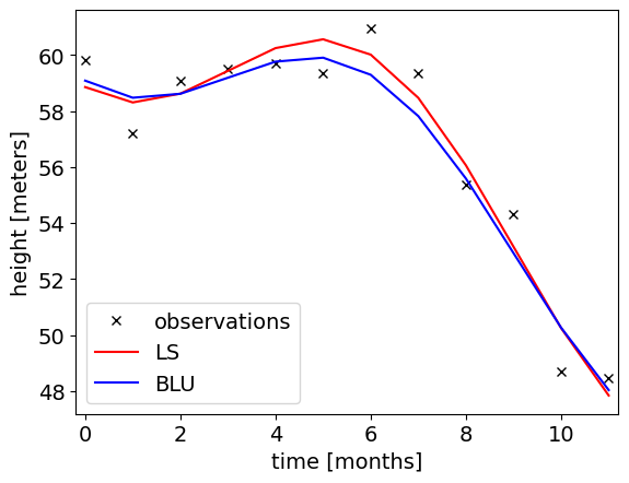
Task 3.1:
- Explain the difference between the fitted models.
- Can we see from this figure which model fits better (without information about the stochastic model)?
Solution 3.1:
- With LS we give equal weight to all observations, while with BLU the first six observations get larger weight and therefore the fitted line is closer to those observations such that the corresponding residuals are smaller.
- By only looking at figure, we cannot conclude which model fits better, since it does not show that some observations are more precise than others. Therefore we often add error bars.
4. Confidence bounds#
In the code below you need to calculate the confidence bounds, e.g., CI_yhat_BLU is a vector with the values \(k\cdot\sigma_{\hat{y}_i}\) for BLUE. This will then be used to plot the confidence intervals:
$\(
\hat{y}_i \pm k\cdot\sigma_{\hat{y}_i}
\)$
Recall that \(k\) can be calculated from \(P(Z < k) = 1-\frac{1}{2}\alpha\).
Task 4.1:
Complete the code below to calculate the 98% confidence intervals of both the observations \(y\) and the adjusted observations \(\hat{y}\) (model values for both LS and BLU).
Use norm.ppf to compute \(k_{98}\). Also try different percentages.
yhat_LS = A @ xhat_LS
Sigma_Yhat_LS = A @ Sigma_xhat_LS @ A.T
yhat_BLU = A @ xhat_BLU
Sigma_Yhat_BLU = A @ Sigma_xhat_BLU @ A.T

alpha = 0.02
k98 = norm.ppf(1 - 0.5*alpha)

CI_y = k98 * np.sqrt(np.diagonal(Sigma_Y))
CI_yhat_LS = k98 * np.sqrt(np.diagonal(Sigma_Yhat_LS))
CI_yhat_BLU = k98 * np.sqrt(np.diagonal(Sigma_Yhat_BLU))
You can directly run the code below to create the plots.
plt.figure(figsize = (10,4))
plt.rc('font', size=14)
plt.subplot(121)
plt.plot(times, y, 'kx', label='observations')
plt.plot(times, yhat_LS, color='r', label='LS')
plt.plot(times, yhat_LS + CI_yhat_LS, 'r:', label=f'{100*(1-alpha):.1f}% conf.')
plt.plot(times, yhat_LS - CI_yhat_LS, 'r:')
plt.xlabel('time [months]')
plt.ylabel('height [meters]')
plt.legend(loc='best')
plt.subplot(122)
plt.plot(times, y, 'kx', label='observations')
plt.errorbar(times, y, yerr = CI_y, fmt='', capsize=5, linestyle='', color='blue', alpha=0.6)
plt.plot(times, yhat_BLU, color='b', label='BLU')
plt.plot(times, yhat_BLU + CI_yhat_BLU, 'b:', label=f'{100*(1-alpha):.1f}% conf.')
plt.plot(times, yhat_BLU - CI_yhat_BLU, 'b:')
plt.xlim(-0.2, (number_of_observations - 1) + 0.2)
plt.xlabel('time [months]')
plt.legend(loc='best');
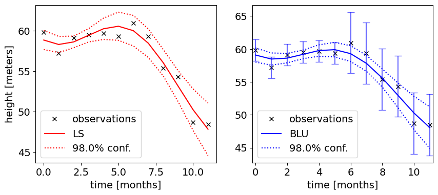
Task 4.2:
Discuss the shape of the confidence bounds. Do you think the model (linear trend + annual signal) is a good choice?
Solution 4.2:
The LS method does not take into account the precision of the observations; this is why there are no error bars plotted on the left figure.
By including the precision of the observations (the error bars in the right figure), as done in the BLU method, you can better assess whether the fit is good.
With BLU: higher precision of first 6 observations, results in tighter confidence intervals as expected.
Similarly as with a linear trend, you can observe a ‘widening’ towards to end, the uncertainty in the fitted model is increasing since there is less ‘support’ from observations on both sides.
Overall the fitted model seems a good choice: it follows the observations nicely and confidence region seems not too wide compared to the fitted model trend.
Task 4.3:
What is the BLU-estimated melting rate and the amplitude of the annual signal and their 98% confidence interval? Hint: extract the estimated values and standard deviations from xhat_BLU and std_xhat_BLU, respectively.
rate = xhat_BLU[1]
CI_rate = k98 * std_xhat_BLU[1]

amplitude = xhat_BLU[2]
CI_amplitude = k98 * std_xhat_BLU[2]

print(f'The melting rate is {rate:.3f} ± {CI_rate:.3f} m/month (98% confidence level)')
print(f'The amplitude of the annual signal is {amplitude:.3f} ± {CI_amplitude:.3f} m (98% confidence level)')
The melting rate is -1.043 ± 0.318 m/month (98% confidence level)
The amplitude of the annual signal is -3.235 ± 1.158 m (98% confidence level)
Task 4.4:
Can we conclude the glacier is melting due to climate change?
Solution 4.4:
- the melting rate is signficant
- however, the seasonal signal is quite large compared to the rate and has large uncertainty
- need much longer time span to draw firm conclusions
By Sandra Verhagen, Delft University of Technology. CC BY 4.0, more info on the Credits page of Workbook.