File import#
import numpy as np
import pandas as pd
import matplotlib.pyplot as plt
import os
from urllib.request import urlretrieve
plt.rcParams.update({'font.size': 14})
Part 0: Download and Import and Interpret the Data Set#
\(\text{Task 7.1:}\)
Complete the code cell below to import the data. Use the commented lines of code to interpret the contents.
def findfile(fname):
    if not os.path.isfile(fname):
        print(f"Downloading {fname}...")
        urlretrieve('http://files.mude.citg.tudelft.nl/'+fname, fname)

findfile('chla.csv')
Downloading chla.csv...
h = pd.read_csv('chla.csv', delimiter=',', header=1)

h.columns=['Date', 'Chlfa']
h.head()
| Date | Chlfa | |
|---|---|---|
| 0 | 3/1/14 1:00 | 7.055628 |
| 1 | 3/1/14 2:00 | 7.018217 |
| 2 | 3/1/14 3:00 | 7.060986 |
| 3 | 3/1/14 4:00 | 7.340142 |
| 4 | 3/1/14 5:00 | 7.717564 |
Unfortunately we can’t create a plot to visualize the data with the Date information because matplotlib doesn’t know how to interpret the value as it’s stored as text.
Part 1: Use Pandas to Plot the Time Series with datetime#
The Pandas method is datetime, which converts the object type from a generic (un-usable-for-plotting) data type ito a datetime type. A full explanation of this is outside the scope of MUDE, so we simply illustrate it below. For our purposes, note that:
the
datetimeobject created byto_datetimeis a significant improvement on the standard Python functionalityPandas provides a lot of methods that can use it (we only scratch the surface here)
to learn more, if you are interested, there is plenty available online, like the tutorial here
\(\text{Task 7.2:}\)
Study the code cell below to see how to create a datetime object. Note in particular the dtype printed in the Pandas output, indicating the method was successful.
h['Date'] = pd.to_datetime(h['Date'], format='%m/%d/%y %H:%M')
h['Date']
0      2014-03-01 01:00:00
1      2014-03-01 02:00:00
2      2014-03-01 03:00:00
3      2014-03-01 04:00:00
4      2014-03-01 05:00:00
               ...
5874   2014-10-31 19:00:00
5875   2014-10-31 20:00:00
5876   2014-10-31 21:00:00
5877   2014-10-31 22:00:00
5878   2014-10-31 23:00:00
Name: Date, Length: 5879, dtype: datetime64[ns]
\(\text{Task 7.3:}\)
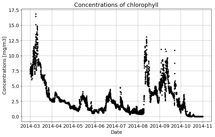
Now you can run the cell below to visualize the data!
plt.figure(figsize=(10, 6))
plt.plot(h['Date'], h['Chlfa'],'k.')
plt.xlabel('Date')
plt.ylabel('Concentrations [mg/m3]')
plt.grid()
plt.title('Concentrations of chlorophyll');
By Tom van Woudenberg and Robert Lanzafame, Delft University of Technology. CC BY 4.0, more info on the Credits page of Workbook.