Analysis of Passing Maneuvers#
Part 1: Introduction and set up#
In this assignment, you will work with data on passing maneuvers from a fixed-based driving simulator experiment (you can read more about it here!) to assess the safety of these maneuvers. This type of analysis is key to better understand conflicts between drivers and better estimate possible crashes.
To do so, you will use data with three random variables:
The speed of the passing vehicle (\(S\), m/s)
Gap from the passing vehicle to the front of the passed vehicle at the end of the maneuver (\(d\), m)
The duration of the pass maneuver (\(P\), s)
import numpy as np
from scipy.stats import multivariate_normal
from scipy.stats import norm
import matplotlib.pyplot as plt
from statistics import mean, stdev
import os
from urllib.request import urlretrieve
def findfile(fname):
    if not os.path.isfile(fname):
        print(f"Downloading {fname}...")
        urlretrieve('http://files.mude.citg.tudelft.nl/'+fname, fname)

findfile('modif_data_passing.csv')
data = np.loadtxt('modif_data_passing.csv', delimiter = ',', skiprows=1)
data
array([[18.18, 11.34,  5.48],
       [26.53, 46.06,  5.25],
       [22.09, 33.28,  2.6 ],
       ...,
       [23.84, 28.21,  6.3 ],
       [21.93, 15.86,  5.01],
       [21.91, 20.64,  5.91]], shape=(1287, 3))
Part 2: Data exploration#
Task 2.1:
Plot the data: have a look at the histograms of each variable as well as the scatter plots of each of them against the others. What can you conclude?
variable_names = ['S', 'd', 'P']
fig, axs = plt.subplots(3, 3, figsize=(8, 6), layout = 'constrained')

for i in range(data.shape[1]):
    for j in range(data.shape[1]):
        if i == j:
            axs[i,j].grid()
            axs[i, j].hist(data[:, i], bins=20, density=True, alpha=0.5, edgecolor='black')
            axs[i, j].set_xlabel(variable_names[i])
            axs[i,j].set_ylabel('PDF')
        if i < j:
            axs[i,j].grid()
            axs[i, j].scatter(data[:, i], data[:, j], alpha=0.5, edgecolor='black')
            axs[i, j].set_xlabel(variable_names[i])
            axs[i, j].set_ylabel(variable_names[j])
        if i > j:
            axs[i, j].axis('off')
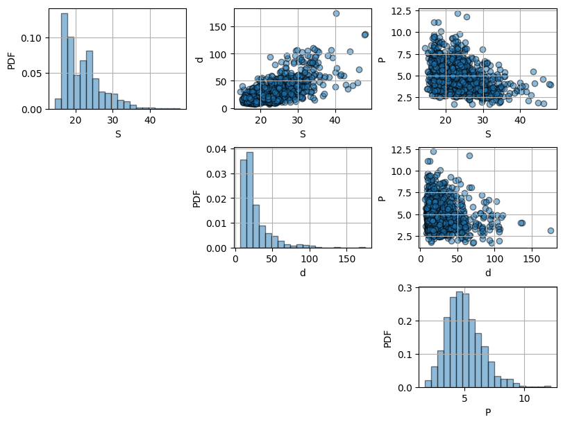
Solution 2.1:
From the histograms, we can see that the three variables seem to be right-skewed as they have a positive tail. This is specially noteworthy for \(S\) and \(d\). From the scatter plots, we can see that \(S\) and \(d\) are positively correlated with a relevant strong correlation, while \(d\) and \(P\) and \(S\) and \(P\) seem to be negatively correlated with a weaker correlation.
Task 2.2:
Quantify the stregth of the correlation between each pair of variables using Pearson’s correlation coefficient. What can you conclude?
def calculate_covariance(X1, X2):
    mean_x1 = mean(X1)
    mean_x2 = mean(X2)
    diff_x1 = [item-mean_x1 for item in X1]
    diff_x2 = [item-mean_x2 for item in X2]
    product = [a*b for a,b in zip(diff_x1,diff_x2)]
    covariance = mean(product)
    return covariance

def pearson_correlation(X1, X2):
    covariance = calculate_covariance(X1, X2)
    correl_coeff = covariance/(stdev(X1)*stdev(X2))
    return correl_coeff

print("Pearson's correlation coefficient between S and d is",
      np.round(pearson_correlation(data[:,0], data[:,1]), 2))

print("Pearson's correlation coefficient between S and P is",
      np.round(pearson_correlation(data[:,0], data[:,2]), 2))

print("Pearson's correlation coefficient between P and d is",
      np.round(pearson_correlation(data[:,1], data[:,2]), 2))
Pearson's correlation coefficient between S and d is 0.68
Pearson's correlation coefficient between S and P is -0.36
Pearson's correlation coefficient between P and d is -0.19
Solution 2.2:
As expected from the first observation of the data, we can see that \(S\) and \(d\) are positively correlated with a reasonably strong correlation of 0.68, while \(S\) and \(P\) and \(d\) and \(P\) are negatively correlated with weaker correlations of -0.36 and -0.19, respectively.
This means, that the higher the speed of the passing vehicle (\(S\)), we can expect a shorter duration of the passing maneuver (\(P\)) and a higher distance from the passing vehicle to the front of the passed vehicle at the end of the maneuver (\(d\)).
Part 3: Multivariate Gaussian distribution#
Task 3.1:
Model the joint distribution of \(S\), \(d\) and \(P\) using a multivariate Gaussian distribution. Follow the steps:
Define the vector of means
Define the covariance matrix
Define the bivariate Gaussian distribution and draw 500 samples to compare with the observations.
Do you see differences between the observations and the samples from the bivariate Gaussian distribution? Compare both the univariate distributions and the bivariate scatter plots.
# Define the vector of means
mu1 = mean(data[:,0])
mu2 = mean(data[:,1])
mu3 = mean(data[:,2])

mu = [mu1, mu2, mu3] #vector of means

# Define the covariance matrix
s1 = stdev(data[:,0])
s2 = stdev(data[:,1])
s3 = stdev(data[:,2])
covariance_12 = calculate_covariance(data[:,0], data[:,1])
covariance_13 = calculate_covariance(data[:,0], data[:,2])
covariance_23 = calculate_covariance(data[:,1], data[:,2])
sigma = np.array([[s1**2 , covariance_12, covariance_13], [covariance_12, s2**2, covariance_23], [covariance_13, covariance_23, s3**2]])

# Draw 500 samples from a bivariate Gaussian distribution
samples = multivariate_normal(mean=mu, cov=sigma).rvs(size=500)

# Plot against observations

fig, axs = plt.subplots(3, 3, figsize=(8, 6), layout = 'constrained')

for i in range(data.shape[1]):
    for j in range(data.shape[1]):
        if i == j:
            axs[i,j].grid()
            axs[i, j].hist(data[:, i], bins=20, density=True, alpha=0.9, edgecolor='darkblue', facecolor = 'none')
            axs[i, j].hist(samples[:, i], bins=20, density=True, alpha=0.5, edgecolor='black',facecolor='orange')
            axs[i, j].set_xlabel(variable_names[i])
            axs[i,j].set_ylabel('PDF')
            axs[i,j].legend(['observations', 'samples'])
        if i < j:
            axs[i,j].grid()
            axs[i, j].scatter(data[:, i], data[:, j], alpha=0.25, edgecolor='darkblue', facecolor='none')
            axs[i, j].scatter(samples[:, i], samples[:, j], alpha=0.5, edgecolor='black',facecolor='orange')
            axs[i, j].set_xlabel(variable_names[i])
            axs[i, j].set_ylabel(variable_names[j])
            axs[i, j].legend(['observations', 'samples'])
        if i > j:
            axs[i, j].axis('off')
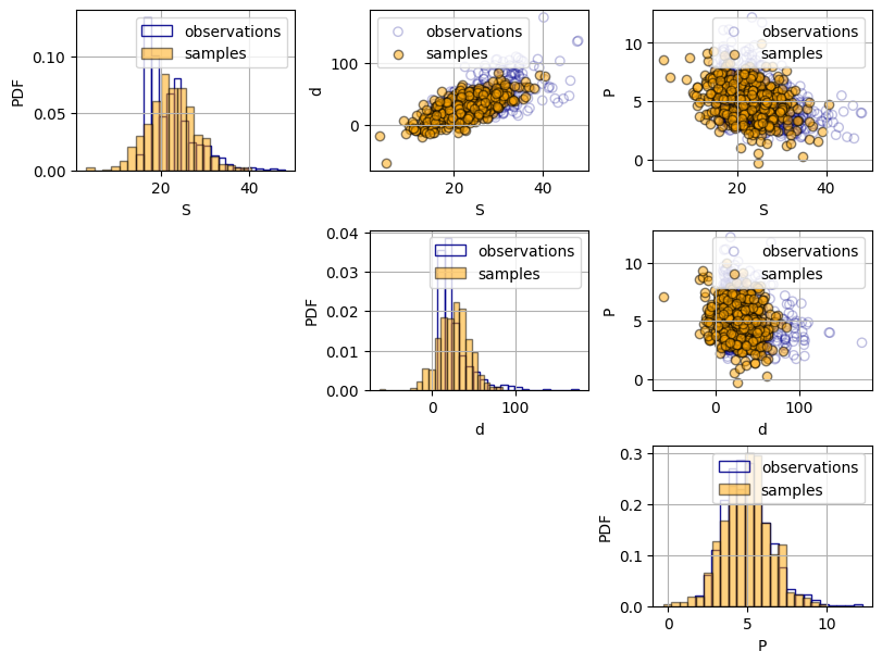
Solution 3.1:
A key property of using a multivariate Gaussian distribution is that both the marginal distributions (the distribution of each of the random variables) and the joint distribution are Gaussian. Therefore, as it can be observed in the histograms, the samples present a symmetric bell-shaped distribution, while the observation have a right tail. This behavior cannot be captured using a Gaussian distribution.
Regarding the bivariate plots, the samples seem to capture the strength of the dependence in the observations, However, the shape of the dependence of the samples is more elliptical, while in some pairs that does not fully hold (e.g.: plot \(S\) and \(P\)).
Task 3.2:
Now that you have a model, you want to get insights into how safe the circulation is on the road you are studying. In previous studies in a similar area, they have defined the following safety thresholds \(^*\):
High speeds lead to reduced driver’s reaction time and increased stopping distances. Therefore, \(S < 30 \ m/s\) is recommended.
Reduced distances between the passing and passed vehicle after the maneuver may indicate more risky maneuvers increasing the chance of collision. Thus, \(d>45 \ m\) is recommended.
Long passing times may lead to dangerous situations as it increases the likelihood of the passing maneuver ending in a no-passing zone due to traffic, road conditions etc. Hence, \(P<7 \ s\) is recommended.
Given the above safety thresholds, what is the probability of meeting them?
Hint: It can be computed analytically similarly to the 2-dimensional case. However, it is easier to use simulations to compute this probability.
\(^*\) These thresholds are not based in actual evidence and are just for academic purposes.
# Draw 10000 samples from the multivariate Gaussian distribution
samples = multivariate_normal(mean=mu, cov=sigma).rvs(size=10000)

# Count number of points that meet the condition
condition = sum(np.logical_and(samples[:, 0] < 30, samples[:, 1] > 45, samples[:,2]<7))

# Compute the probability of the condition
prob_meeting_condition = condition / 10000
print(f"The probability of meeting the safety limits (S < 30, d > 45 and P < 7) is approximately {prob_meeting_condition:.4f}")
The probability of meeting the safety limits (S < 30, d > 45 and P < 7) is approximately 0.1117
Part 4: Conditionalizing the multivariate Gaussian distribution#
Task 4.1:
You have now installed a sensor that measures the distance between the passed and passing vehicle at the end of the maneuver (\(d\)). For a passing vehicle, \(d=53 \ m\). What is the probability that it was a safe maneuver?
To answer the question, follow the steps:
Compute the distribution of \(S\) and \(P\) given \(d=53 \ m\).
Compute the probability of \(P(S \leq 30 \ m/s, P \leq 7 \ s|d=53 \ m)\).
Solution 4.1:
One of the properties of the multivariate Gaussian distribution is that, when we conditionalize, we always obtain another Gaussian distribution. Here, we are working with a 3-dimensional distribution and we are conditionalizing on one variable (\(d\)). Therefore, we will obtain a bivariate Gaussian distribution for \(S\) and \(P\). But which one?
We can compute the (new) parameters of the conditional distribution of \(S\) and \(P\) using the following expressions (note that they assume that the conditioning variable is \(X_3\) (the third variable in the expressions below)):
Note that the covariance matrix for the conditioned distribution reduces to the conditional variance of \(S\) and \(P\). This is because we have a bivariate distribution, so given the value of one variable, the resulting conditional distribution is univariate. However, if we had been working with a distribution of 3 variables, when conditionalizing in one, we would have obtained a conditional bivariate distribution.
# Compute the parameters of the conditional distribution
cond_mu_vector = np.array([22.2, 5.0]) + np.multiply(np.multiply(np.array([69.5, -5.2]), (19**2)**(-1)),(53 - 26.1))
cond_sigma_matrix = np.array([[5.3**2, -2.8], [-2.8,  1.5**2]]) - np.multiply(np.multiply(np.array([69.5, -5.2]), (19**2)**(-1)), np.array([[69.5], [-5.2]]))

# Compute the conditional probability
cond_prob = multivariate_normal(mean=cond_mu_vector, cov=cond_sigma_matrix).cdf([30, 7])
print('The conditional probability of S < 30 and P < 7 given d = 53 is approximately {:.4f}'.format(cond_prob))
The conditional probability of S < 30 and P < 7 given d = 53 is approximately 0.7044
Task 4.2:
Using the results of the previous task, compare the conditional and unconditional distributions of \(S\) and \(P\). To do so, follow the next steps:
Plot the conditional and unconditional univariate marginal distributions of \(S\) and \(P\).
Plot the contours of the PDF of the conditional and unconditional joint distributions of \(S\) and \(P\).
Explain the differences in terms of both the location and the width of the distribution.
# Compare the conditional and unconditional margins

# Evaluate both the conditional and unconditional univariate PDFs of S and P
values_S = np.linspace(0, 50, 100)
uncond_S_pdf = norm.pdf(values_S, loc = mu1, scale = s1)
cond_S_pdf = norm.pdf(values_S, loc = cond_mu_vector[0], scale = cond_sigma_matrix[0,0]**(0.5))

values_P = np.linspace(0, 15, 100)
uncond_P_pdf = norm.pdf(values_P, loc = mu3, scale = s3)
cond_P_pdf = norm.pdf(values_P, loc = cond_mu_vector[1], scale = cond_sigma_matrix[1,1]**(0.5))

# Plot both PDFs
fig, ax = plt.subplots(1, 2, figsize=(8, 4), layout = 'constrained')
ax[0].plot(values_S, uncond_S_pdf, 'k', label = 'Unconditional distribution')
ax[0].plot(values_S, cond_S_pdf, '--k', label = 'Conditional distribution')
ax[0].grid()
ax[0].set_xlabel('pdf')
ax[0].set_xlabel('${S}  [m/s]$')
ax[0].legend();

ax[1].plot(values_P, uncond_P_pdf, 'k', label = 'Unconditional distribution')
ax[1].plot(values_P, cond_P_pdf, '--k', label = 'Conditional distribution')
ax[1].grid()
ax[1].set_xlabel('pdf')
ax[1].set_xlabel('${P}  [m]$')
ax[1].legend();
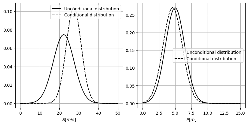
Solution 4.2a:
In the plots above, it is possible to see the influence of the conditionalization in the univariate marginals, \(S\) and \(P\). We have conditionalized \(d\) in a value above its mean. Since the correlation between \(d\) and \(S\) is positive, the distribution of \(S\) moves towards positive values; increasing values of \(d\) imply also higher values of \(S\). Also, the conditional distribution of \(S\) becomes narrower as the model has more information.
On the other hand, \(P\) is not strongly correlated to \(d\), presenting a weak negative correlation (\(\rho_{d,P}=-0.19\)). Therefore, the marginal distribution does not suffer a change as noteworthy as the distribution of \(S\). Although it is difficult to distinguish from the plot, the standard deviation of \(P\) gets slightly reduced and the distribution shifts towards negative values; increasing values of \(d\) imply decreasing values of \(P\).
# Compare the joint conditional and unconditional distribution

# Define the mesh of values where we want to evaluate the random variables
#already done in previous cell

# Define the grid
X1,X2 = np.meshgrid(values_S,values_P)
X = np.array([np.concatenate(X1.T), np.concatenate(X2.T)]).T

# Evaluate the CDF
Z_uncond = multivariate_normal(mean=[mu[0], mu[2]], cov=[[sigma[0][0], sigma[0][2]],[sigma[2][0], sigma[2][2]]]).pdf(X)
Z_cond = multivariate_normal(mean=cond_mu_vector, cov=cond_sigma_matrix).pdf(X)

# Create contours plot
levels = np.linspace(0, 0.025, 11)
fig = plt.figure(figsize=(7,5), layout= 'constrained')
ax = fig.add_subplot(111)
contours = ax.contour(X1, X2, Z_uncond.reshape(X1.shape).T, levels, cmap='YlGnBu', vmin=0, vmax = 0.025)
contours2 = ax.contour(X1, X2, Z_cond.reshape(X1.shape).T, levels, cmap='Greys', vmin=0, vmax = 0.025)
ax.grid()
ax.set_xlim([0, 50])
ax.set_ylim([1, 9])
ax.set_xlabel('${S} [m/s]$')
ax.set_ylabel('${P} [s]$')
fig.colorbar(contours, ax=ax, label='Unconditional joint PDF')
fig.colorbar(contours2, ax=ax, label = 'Conditional joint PDF');
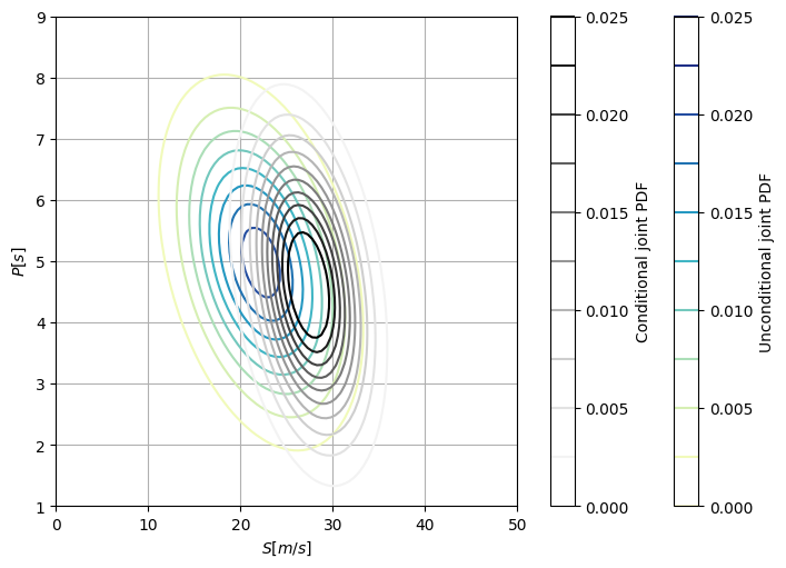
Solution 4.2b
You can also see how, similarly to the marginal plots, the mean of \(P\) slightly moves towards lower values when conditionalizing due to the negative correlation between \(D\) and \(P\). On the contrary, the mean of \(S\) significantly moves towards higher values due to the stronger positive correlation between \(S\) and \(D\).
By Patricia Mares Nasarre, Delft University of Technology. CC BY 4.0, more info on the Credits page of Workbook.