Report#
Questions for Part 2. Data exploration#
2.1 How are the variables related to each other? Comment on the strength of the dependence and report quantitative values. (1 point)
\(S\) and \(D\) are positively correlated with a reasonably strong correlation of 0.68, while \(S\) and \(P\) and \(D\) and \(P\) are negatively correlated with weaker correlations of -0.36 and 0.19, respectively. This means, that the higher the speed of the passing vehicle (\(S\)), we can expect a shorter duration of the passing maneuver (\(P\)) and a higher distance from the passing vehicle to the front of the passed vehicle at the end of the maneuver (\(D\)).
Grading scheme (1 point):
Reporting correct values of the correlation coefficients: 0.5 points
Right interpretation of those values: 0.5 points
Questions for Part 3. Multivariate Gaussian distribution#
3.1 How appropriate is the multivariate Gaussian distribution to model the joint distribution of the data? Comment both on the marginal distributions and the dependence between variables. You may want to use plots to illustrate your arguments. (2 points)
A key property of using a multivariate Gaussian distribution is that both the marginal distributions (the distribution of each of the random variables) and the joint distribution are Gaussian. Therefore, as it can be observed in the histograms in the Figure below, the samples present a symmetric bell-shaped distribution, while the observation have a right tail. This behavior cannot be captured using a Gaussian distribution.
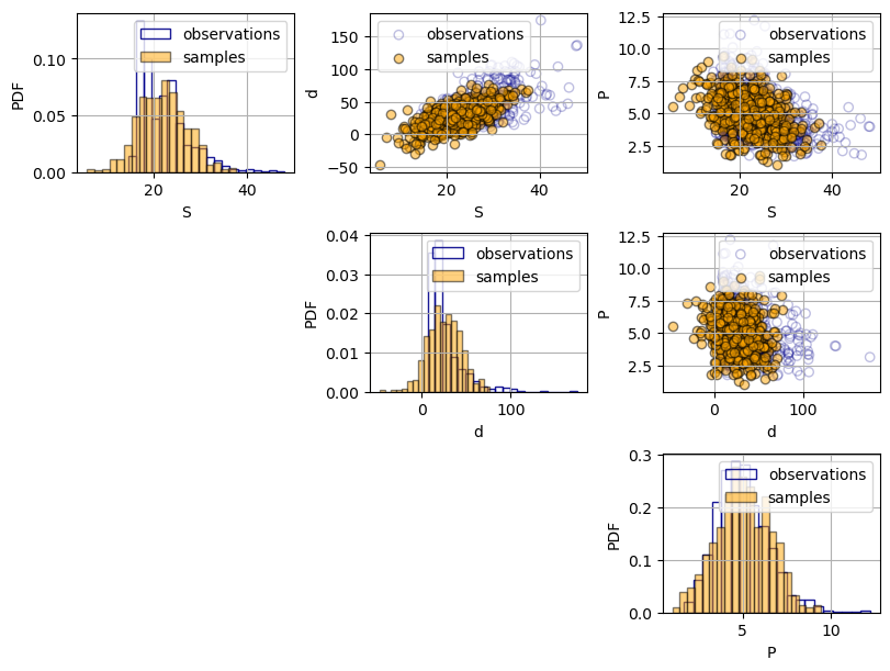
Regarding the bivariate plots, the samples seem to capture the strength of the dependence in the observations, However, the shape of the dependence of the samples is more elliptical, while in some pairs that does not fully hold (e.g.: plot \(S\) and \(P\)).
Grading scheme (2 points):
Correct comparison of the univariate distributions, tail in the histograms: 1 point
Correct comparison of the scatter plots: 1 point
If partially correct comparison of scatter plots (e.g.: strength of dependence seems ok): 0.5
3.2 Assuming the safety thresholds \(S<30m/s\), \(D>45m\) and \(P<7s\), what is the probability of doing a passing maneuver under safe conditions? What is the difference between assuming independence or accounting for it using the multivariate Gaussian distribution? (1.75 points)
The probability of meeting the safety limits (S < 30, D > 45 and P < 7) using the multivariate Gaussian distribution is approximately 0.12 and assuming independence is 0.14.
The difference in this case is not major, although assuming independence is in the unsafe side, as it assumes it is more likely to be driving under safe conditions.
Grading scheme (1.75 points):
Correct computation of the probability using multivariate Gaussian: 0.75 points
Correct computation of the probability assuming independence: 0.75 points
Appropriate comments on the differences: 0.25 points
Questions for Part 4. Conditionalizing the multivariate Gaussian distribution#
4.1 Given that you have observed a driver passing with D=53 m, what is the probability of that maneuver being safe? What is the difference between assuming independence and modeling dependence using the multivariate Gaussian distribution? (1.75 points)
The conditional probability of S < 30 and P < 7 given D = 53 using the multivariate Gaussian distribution is approximately 0.70 while assuming independence is 0.85.
Similarly to the unconditional probabilities, assuming independence is in the unsafe side, as it assumes it is more likely to be driving under safe conditions.
Grading scheme (1.75 points):
Correct computation of the probability using multivariate Gaussian: 0.75 points
Correct computation of the probability assuming independence: 0.75 points
Appropriate comments on the differences: 0.25 points
4.2 How does the distribution change when conditionalizing in D = 53 m? You may want to report quantitative values of the parameters and use plots to support your arguments. (2.5 points)
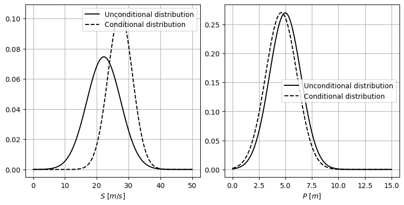
We have conditionalized \(d\) in a value above its mean. Since the correlation between \(d\) and \(S\) is positive, the distribution of \(S\) moves towards positive values; increasing values of \(d\) imply also higher values of \(S\). Also, the conditional distribution of \(S\) becomes narrower as the model has more information.
On the other hand, \(P\) is not strongly correlated to \(d\), presenting a weak negative correlation (\(\rho_{d,P}=-0.19\)). Therefore, the marginal distribution does not suffer a change as noteworthy as the distribution of \(S\). Although it is difficult to distinguish from the plot, the standard deviation of \(P\) gets slightly reduced and the distribution shifts towards negative values; increasing values of \(d\) imply decreasing values of \(P\).
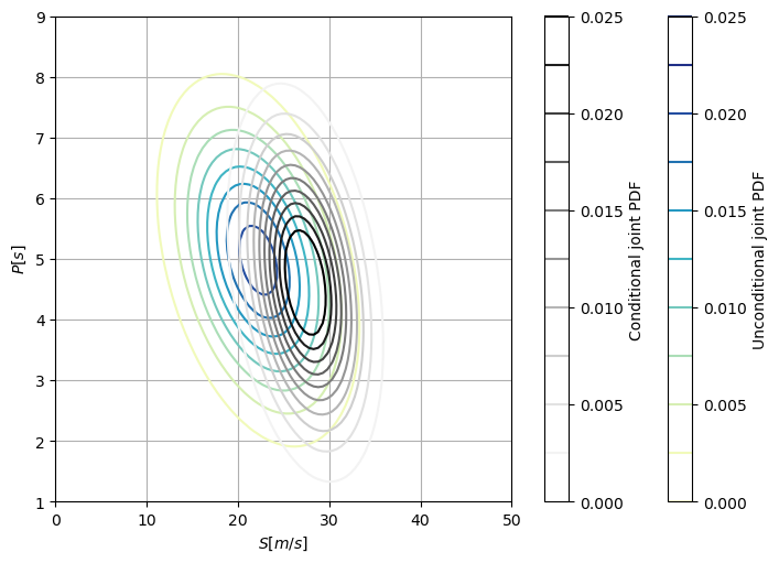
Overall, it is possible to see that the conditional PDF (in greys) is narrower than the unconditional PDF (in colors) as we have provided the model with additional information, thus, reducing the uncertainty. This is especially noteworthy in the \(S\)-dimension.
You can also see how, similarly to the marginal plots, the mean of \(P\) slightly moves towards lower values when conditionalizing due to the negative correlation between \(D\) and \(P\). On the contrary, the mean of \(S\) significantly moves towards higher values due to the stronger positive correlation between \(S\) and \(D\).
This can also be observed in the change of the parameters of the distribution, as shown in the Table below.
Variable |
Unconditional parameters |
Conditional parameters |
|---|---|---|
S |
(22.2, 5.4) |
(27.4, 3.8) |
P |
(5.0, 1.48) |
(4.6, 1.47) |
Grading scheme (2.5 points):
Correct computation of the conditional distribution (computation of the conditional parameters): 0.5 points
Correct interpretation of the change in the univariate conditional distributions: 1 point
Correct interpretation of the change in the bivariate conditional distributions: 1 point
By Patricia Mares Nasarre, Delft University of Technology. CC BY 4.0, more info on the Credits page of Workbook.