Report#
Part 1#
For part 1, Try splitting into pairs within your group and each choose a model to consider, then after a few minutes regroup and explain your results to each other. Please refer to the book if you are unsure about any terms.
The question below refers to the 4 examples in Part 1 of the notebook.
1.1 Classify the models in the examples using the categories in the textbook. Please provide an explanation of your choice.
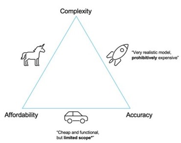
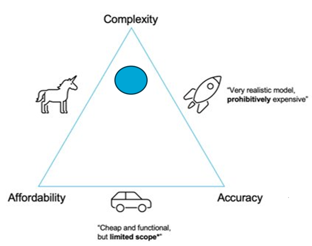
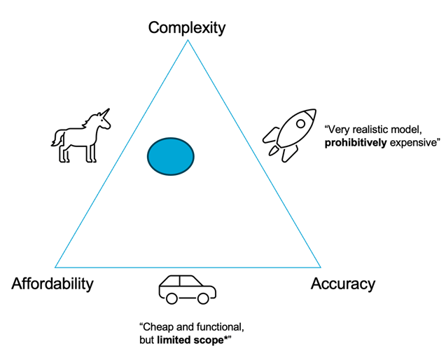
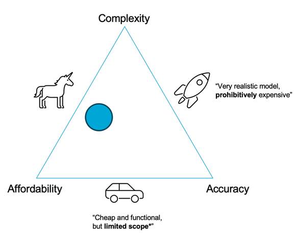
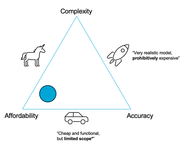
1.2 Place each model on the tradeoff triangle (shown below) and provide an explanation of your choice.
1.3 What simplifications are made in the models?
1.4 What types of uncertainty are the models affected by?
The following solutions are for questions 1.1, 1.2, 1.3 and 1.4, per model:
All models are subject to all the types of uncertainty that we have defined in the book. As we are modelling a natural process they are all highly susceptible to randomness (Epistemic). Aleatoric uncertainty comes in as we are only able to capture so much of the natural system. We often have to make simplifications of the natural world, so the knowledge of the system is limited. Lastly, all the data gathered will be subject to some kind of error, be it human error or instrument error.
Model 1
Global climate models are mostly phenomenological, based on atmospheric physics and observed data. While they may include some mechanistic parts, accuracy is limited due to the use of grid-based numerical methods like finite element or finite difference. Their complexity is high because of numerical challenges.
Stochastic elements are sometimes added to handle uncertainty but are often avoided. Instead, many ensemble simulations are run to assess variability.
Heat exchange is usually modeled phenomenologically—static and deterministic, though mechanistic models like diffusion equations are possible.
River discharge may be modeled using data or simplified physics, typically ignoring geometry, non-linear, or time-dependent effects.
Ice melting is generally treated as a static, time-invariant process.
Some simplifications:
Treats the climate system in terms of broad averages and ignores local effects
Simplifies precipitation and discharge processes to outputs of energy balance.
Treats ice melt as a direct consequence of heat/precipitation.
Model 2
Solar heat can be modeled deterministically using mechanistic equations, accounting for daily and seasonal cycles. While complex, a stochastic model could simplify this variability.
Snow and ice cover can be estimated from historical data using stochastic or regression models. These are often time-invariant, non-linear, and static, but can feed into mechanistic models to estimate river temperature and ice melting rates, which are typically modeled as deterministic and time-invariant.
River discharge is well-documented and could support more complex, non-linear, and even dynamic models. While ice melting can often be simplified as static (assuming stable temperature), discharge is better modeled dynamically due to rapid changes caused by rain or melting events.
Some simplifications:
Treats the climate system in terms of broad averages and ignores local effects
Considers only heat balance, neglecting other feedbacks (wind, vegetation, permafrost).
River temperature and discharge are simplified to direct outcomes of snowmelt + rainfall.
Model 3
Discharge and temperature will likely come from data and could be modeled stochastically using probability distributions.
The model for ice melting in the river could be mechanistic (involving ice mass, heat capacity, and water temperature), but is more likely phenomenological—possibly using dimensionless analysis due to complex river geometry.
The rope tension and catenary shape should be modeled mechanistically, and are clearly non-linear. This is likely a static problem, since the load builds slowly as ice melts. However, if there’s a sudden surge in river flow or ice breakage, it might become a dynamic impulse load.
Some simplifications:
Focuses only on 1 km upstream of Nenana.
Assumes river discharge and temperature alone determine ice melt.
Ice deformation simplified to deterministic link between melt and mechanical response.-
Model 4
See the solution for Model 3. In this case, a deliberate decision was made to abandon complex mechanistic and phenomenological models for ice deformation. Instead, the model focuses on estimating the probability of reasonable outcomes.
According to the accuracy-complexity-cost triangle, this approach sacrifices some accuracy, but significantly reduces complexity and improves affordability.
Some simplifications:
Ice modeled as uniform continuum, so it ignores sudden break-up dynamics, irregular block movement, or jamming.
Rope tension linked deterministically to velocity, not considering unexpected load paths.
Part 2#
Before answering these questions, please work through Part 2 of the notebook.
2.1 For model 1, what does the coefficient of determination \(R^2\) tell you?. What can you conclude from this?
Coefficient of determination \(R^2\) measures the percentage of the variance in our observations explained by the model. Thus, the higher, the better. As we can see, the value of \(R^2\) is quite low. Only ≈15% of the variance is explained by the model, which is very low. Therefore, the linear model is not able to explain the scatter in our observations.
2.2 For model 1, describe the resulting two plots. What can you conclude from this?
In the first plot, we observe that the observations have a high scatter around the fitted line. In the second plot, we compare the observations with the predictions of the model. The perfect fit would correspond to the 45-degrees line in black. Thus, the model has a poor performance.
2.3 For model 1, what can you conclude from looking at the error bars? Would you have confidence in this model?
If you consider that you need to place a bet with not only the day but also the hour and minute at which the ice would break, the model is not accurate enough. You can see that the confidence interval spans almost 20 days!
2.4 For model 2, please describe the resulting two plots. What can you conclude from this? Looking at the error bars, would you have confidence in this model?
For model 2, we see very similar things to model 1. Firstly, there is a high degree of scatter around the fitted line. When comparing the observations with the predictions of the model there is still no discernible fit around the 45-degree line. Again, the error bars show an interval of about 20 days, nowhere precise enough to place a confident bet.
2.5 Which model, if any, do you think is better according to Goodness of Fit metrics? Why?
Neither! They are both bad.
Part 3#
3.1 (Optional but recommended) Based on these models and the data you have available, make a prediction for the ice breakup for next year!
Most groups recognized the importance of discharge and ice thickness and found really interesting ways to connect observable variables to these, which are at the core of the prediction model. Some were more complex than others, and ranged in scale from global to regional, but all incorporated interesting aspects of hydrology, climate, weather, etc. (solar radiation, for example, was a nice one, as it has complex relationship with snow/ice melting, both on the river and upstream in the watershed). Ideally one would “observe” the discharge and ice thickness at breakup to identify a critical threshold of discharge that may cause the ice to break, given the current ice thickness. This is a great idea; however, it is much more difficult to do in practice.
We note that:
It is impossible to measure ice thickness during breakup. Also, at some point before breakup occurs it becomes unsafe to measure the ice thickness. You can get around this issue by using the Ashton model to estimate ice thickness (extrapolate from last measurements).
There will be “scatter” in the relationship between discharge and ice thickness, it is not a perfect 1:1 relationship.
To make the bet, we are making a prediction (extrapolating). We need to predict discharge and thickness, both of which are heavily dependent on weather, which is very difficult to predict accurately, especially when we need to look several weeks in advance! This makes the ice classic a very challenging (but interesting) modelling problem.
3.2 (Optional but recommended) Outline your own conceptual model based on what you have learned in the notebook. Explain your choices.
This one is up to you :)
Jialei Ding and Robert Lanzafame, Delft University of Technology. CC BY 4.0, more info on the Credits page of Workbook.