An Elastically Supported Rod

Part 1: A modification to the PDE: continuous elastic support

In the book, the finite element derivation and implementation of rod extension (the 1D Poisson equation) is presented. In this workshop, you are asked to do the same for a slightly different problem.

For this exercise we consider an elastically supported rod. An example of this would be a foundation pile in soil. The equilibrium of an elastically supported rod can be described with the following differential equation:

\[ -EA \frac{\partial^2 u}{\partial x^2} + ku = q \]

where \(EA\) is the axial stiffness of the rod, \(u(x)\) is the unknown displacement, \(k\) is the stiffness of the elastic support and \(q\) is a distributed load. We consider a case with Dirichlet boundary condition at \(x=0\) and a Neumann boundary condition at \(x=L\).

\[\begin{split} u = 0, \quad \text{at} \quad x = 0 \\ EA\frac{\partial u}{{\partial x}} = F, \quad \text{at} \quad x = L \end{split}\]

This differential equation is the inhomogeneous Helmholtz equation, which also has applications in dynamics and electromagnetics.

The finite element discretized version of this PDE can be obtained following the same steps as shown for the unsupported rod in the book. The additional term with respect to the case without elastic support is the second term on the left hand side: \(ku\). Using Neumann boundary condition (i.e. an applied load) at \(x=L\), the following expression is found for the discretized form:

\[\left[\int \mathbf{B}^T EA \mathbf{B} + \mathbf{N}^T k \mathbf{N} \,dx\right]\mathbf{u} = \int \mathbf{N}^T q \,d x + \mathbf{N}^T F \Bigg|_{x=L} \]

Task 1.1: Derive the discrete form

Derive the discrete form of the PDE given above. You can follow the same steps as in the book for the term with \(EA\) and the right hand side, but now carrying along the additional term \(ku\) from the PDE. Note that there are no derivatives in this term \(ku\) which means that integration by parts does not need to be applied on it. Show that this term leads to the \(\int\mathbf{N}^Tk\mathbf{N}\,dx\) term in the \(\mathbf{K}\)-matrix.

Solution

Including the additional term resulting from the distributed spring \(ku\), the following differential equation is obtained:

\[-EA \frac{\partial^{2} u}{{\partial x}^{2}} + ku = f\]

The differential equation is rewritten in the weak form by multiplying both sides of the equations by the weight function \(w(x)\) and integrating over the domain.

\[ -\int_{0}^{L} wEA \frac{\partial^{2} u}{\partial x^{2}}\,dx + \int_0^Lwku\,dx = \int_0^Lwf\,dx \quad\forall\quad w\]

Integration by parts is applied, but only to the \(EA\)-term. Neumann boundary conditions are subsdstituted in the boundary term that arises from integration by parts:

\[ \int_{0}^{L} \frac{\partial{w}}{\partial x}EA \frac{\partial u}{\partial x}\,dx + \int_0^Lwku\,dx = \int_0^Lwf\,dx+w(L)F \quad\forall\quad w\]

Next, we discretize the displacement and weight functions:

\[ u^h(x) = \mathbf{Nu} \]

\[ w^h(x) = \mathbf{Nw} \]

We substitute the discretized solution \(u^h\) and the discretized weight function \(w^h\) into the weak form equation. Since the equation has to hold for all \(w\), the term for the distributed spring becomes:

\[ \int_{0}^{L} \mathbf{Bw}EA \mathbf{Bu}+\mathbf{Nw}k\mathbf{Nu}\,dx = \int_0^L \mathbf{Nw}f\,dx+\mathbf{N}(L)\mathbf{w}F \]

We take \(\mathbf{u}\) and \(\mathbf{w}\) out of the integral and eliminiate \(\mathbf{w}\) to get the expression given above (just before the green box in Task 1).

Part 2: Modification to the FE implementation

The only change with respect to the procedure as implemented in the book is the formulation of the \(\mathbf{K}\)-matrix, which now consists of two terms:

\[ \mathbf{K} = \int \mathbf{B}^TEA\mathbf{B} + \mathbf{N}^Tk\mathbf{N}\,dx \]

To calculate the integral exactly we must use two integration points.

\[ \mathbf{K_e} = \sum_{i=1}^{n_\mathrm{ip}} \left(\mathbf{B}^T(x_i)EA\mathbf{B}(x_i) + \mathbf{N}^T(x_i) k\mathbf{N}(x_i) \right) w_i\]

Task 2.1: Code implementation

The only change needed with respect to the implementation of the book is in the calculation of the element stiffness matrix. Copy the code from the book and add the term related to the distributed support in the right position.

Remarks:

• The function evaluate_N is already present in the code in the book

• The get_element_matrix function already included a loop over two integration points

• You need to define \(k\) somewhere. To allow for varying \(k\) as required below, it is convenient to make \(k\) an additional argument of the simulate function and pass it on to lower level functions from there (cf. how \(EA\) is passed on)

import numpy as np
import matplotlib.pyplot as plt

def evaluate_N(x_local, dx):
    return np.array([[1-x_local/dx, x_local/dx]])

def evaluate_B(x_local, dx):
    return np.array([[-1/dx, 1/dx]])

def get_element_matrix(EA, k, dx):  # receive k as parameter
    
    integration_locations = [(dx - dx/(3**0.5))/2, (dx + dx/(3**0.5))/2]
    integration_weights = [dx/2, dx/2]
    n_ip = len(integration_weights)

    n_node = 2
    K_loc = np.zeros((n_node,n_node))

    for x_i, w_i in zip(integration_locations, integration_weights):
        B = evaluate_B(x_i, dx)
        N = evaluate_N(x_i, dx)
        K_loc += EA * B.T @ B * w_i 
        K_loc += k * N.T @ N * w_i  # add stiffness contribution from k

    return K_loc

def get_element_force(q, dx):
    n_node = 2
    N = np.zeros((1,n_node))
    
    integration_locations = [(dx - dx/(3**0.5))/2, (dx + dx/(3**0.5))/2]
    integration_weights = [dx/2, dx/2]
    
    f_loc = np.zeros(n_node)
    
    for x_i, w_i in zip(integration_locations, integration_weights):
        N = evaluate_N(x_i,dx)
        f_loc += N.squeeze()*q*w_i

    return f_loc

def get_nodes_for_element(ie):
    return np.array([ie,ie+1])


def assemble_global_K(rod_length, n_el, EA, k):   # receive k as parameter
    n_DOF = n_el+1
    dx = rod_length/n_el
    K_global = np.zeros((n_DOF, n_DOF))
    
    for i in range(n_el):
        elnodes = get_nodes_for_element(i)
        K_global[np.ix_(elnodes,elnodes)] += get_element_matrix(EA, k, dx)  # pass k to element matrix function
    
    return K_global

def assemble_global_f(rod_length, n_el, q):
    n_DOF = n_el+1
    dx = rod_length/n_el
    f_global = np.zeros(n_DOF)
    
    for i in range(n_el):
        elnodes = get_nodes_for_element(i) 
        f_global[elnodes] += get_element_force(q, dx)
        
    return f_global


def simulate(n_element,
             length=3,
             EA=1e3,
             k=100,        # additional parameter
             F_right=10,
             q_load=-10
    ):

    n_node = n_element + 1

    dx = length/n_element
    x = np.linspace(0,length,n_node)

    K = assemble_global_K(length, n_element, EA, k)  # pass k to assembly function

    f = assemble_global_f(length, n_element, q_load)

    f[n_node-1] += F_right

    u = np.zeros(n_node)

    K_inv = np.linalg.inv(K[1:n_node, 1:n_node])
    u[1:n_node] = np.dot(K_inv, f[1:n_node])

    return x, u

Task 2.2: Analyze the influence of \(k\) on the results

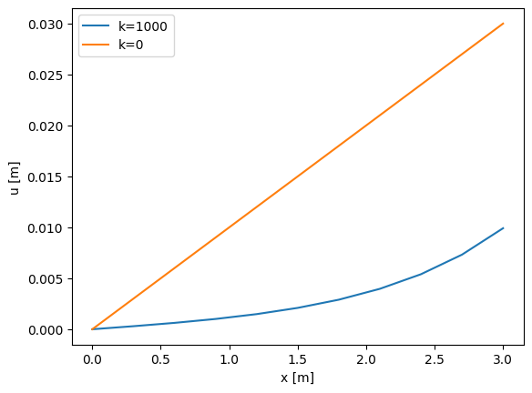
Use the following parameters: \(L=3\text{ m}\), \(EA=1000\text{ N}\), \(F=10\text{ N}\), \(q=0 \text{ N/m}\) (all values are the same as in the book, except for \(q\)). Additionally, use \(k=1000\) N/m² and a discretization of 10 elements.

Check the influence of the distributed support on the solution:

• First use \(q=0\) N/m and \(k=1000\) N/m²

• Then set \(k\) to zero and compare the results

• Does the influence of the distributed support on the solution make sense?

# use the simulate function to get displacements
x10, u_with_k = simulate ( 10, q_load=0, k=1000 )
x10, u_without_k = simulate ( 10, q_load=0, k=0 )

# plot u versus x for both cases
plt.figure()
plt.plot(x10, u_with_k, label='k=1000')
plt.plot(x10, u_without_k, label='k=0')
plt.xlabel('x [m]')
plt.ylabel('u [m]')
plt.legend()
plt.show()

Solution

The solution with \(k=0\) is linear, the PDE says the second derivative must be equal to zero. First derivative follows from the boundary condition on the right as \(du/dx=F/EA\), while displacement at the left is zero through the other boundary condition \(u(0)=0\). This is the expected solution for an axially loaded bar without distributed load.

The solution with \(k>0\) has is nonlinear. Displacements are smaller overall because of the additional resistance from the elastic support. Displacement at \(x=0\) and slope at \(x=L\) are the same as for the solution with \(k=0\) because boundary conditions have not changed.

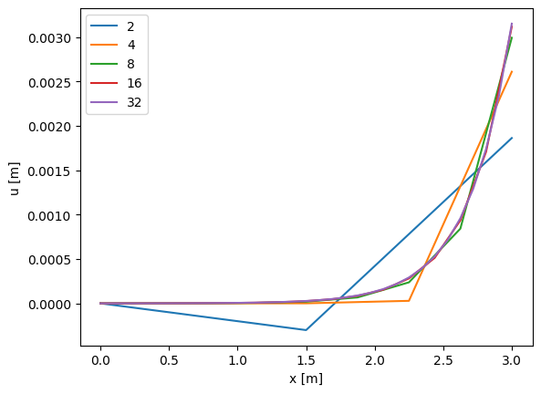
Task 2.3: Investigate the influence of discretization on the quality of the solution

• How many elements do you need to get a good solution with \(k=1000\) N/m?

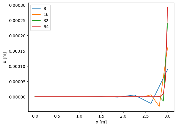
• How about when the stiffness of the distributed support is increased to \(k=10^6\) N/m² ?

Simulate and plot results for different numbers of elements for each of the above questions.

plt.figure()
for n in [2,4,8,16,32]:
    x,u = simulate(n, k=10000, q_load=0)
    plt.plot(x,u,label=str(n))
plt.xlabel('x [m]')
plt.ylabel('u [m]')
plt.legend()
plt.show()


plt.figure()
for n in [8,16,32,64]:
    x,u = simulate(n, k=1e6, q_load = 0)
    plt.plot(x,u,label=str(n))
plt.xlabel('x [m]')
plt.ylabel('u [m]')
plt.legend()
plt.show

<function matplotlib.pyplot.show(close=None, block=None)>

Solution

With \(k=1000\), the solution is already quite accurate with 8 elements and even smoother with 16 elements, while with \(k=10^6\), the solution with 20 elements is still poor. Here something between 32 to 64 elements is needed for a smooth solution. The reason is that there is a very small region with high gradients in the solution with \(k=10^6\), which requires a fine mesh to be resolved. A non-uniform discretization would also be an appealing option here but that would require a bit more coding.

Part 3: Change boundary condition

Now suppose the end of the rod at \(x=L\) is loaded not by a force but by a prescribed displacement. What do you need to change to the simulate function to achieve this? Hint: look at the box Eliminiation of Dirichlet boundary conditions on the Finite element implementation page in the book for a description of how to deal with inhomogeneous Dirichlet boundary conditions in a more general case.

Task 3.1: Implement changes required to prescribe \(u(L)\)

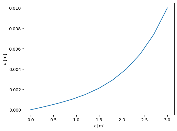
• Code the simulate_new function below such that a nonzero Dirichlet boundary condition is applied at \(x=L\) instead of a force

• Perform the simulation with the same parameters as before and \(k=1000\) and \(u_\mathrm{right}=0.01\) m.

• Compare the obtained field \(u(x)\) to that from task 2.2.

def simulate_new(n_element,
                 length=3,
                 EA=1e3,
                 k=1000,
                 u_right=0.01,
                 q_load=-10
    ):

    n_node = n_element + 1

    dx = length/n_element
    x = np.linspace(0,length,n_node)

    K = assemble_global_K(length, n_element, EA, k)

    f = assemble_global_f(length, n_element, q_load)
    u = np.zeros(n_node)
    u[-1] = u_right

    f_free = f[1:-1] - K[1:-1,-1]*u_right
    K_inv = np.linalg.inv(K[1:-1, 1:-1])
    u[1:-1] = np.dot(K_inv, f_free)

    return x, u

x,u = simulate_new(10, q_load=0, u_right=0.01)
plt.plot(x,u)
plt.xlabel('x [m]')
plt.ylabel('u [m]')

Text(0, 0.5, 'u [m]')

Solution

With the additional nonzero Dirichlet boundary condition, one more row and column need to be removed from the matrix and the right hand side vector needs to be modified. Results are very similar to those obtained in Task 2.2 as they should be because the prescribed displacement at \(x=L\) is close to the one obtained with \(F=10\) N.

By Frans van der Meer, Delft University of Technology. CC BY 4.0, more info on the Credits page of Workbook.