Functional programming#
import numpy as np
import matplotlib.pyplot as plt
Coding the solver#
We will first code the algorithm above by writing a run_diffusion function that takes all necessary arguments.
def run_diffusion(
    L,       # length of the bar
    dx,      # discretization in space
    dt,      # discretization in time
    kappa,   # heat diffusivity
    T_init,  # initial temperature
    T_left,  # Temperature on the left
    h_right, # Flux on the right
    n_steps, # number of time steps
):
    assert kappa*dt/dx/dx<=0.5, 'Stability condition not satisfied'

    # spatial discretization
    x = np.arange(0, L+dx, dx)
    nx = len(x)

    # solution vectors
    T = np.zeros((n_steps,nx))

    # temperature field at t=0
    T[0,:] = T_init

    # loop through time
    for n in range(n_steps-1):
        # solution on the left
        T[n+1,0] = T_left

        # solution in the interior
        for m in range(1,nx-1):
            T[n+1,m] = T[n,m] + kappa*dt/dx/dx * (T[n,m+1]-2*T[n,m]+T[n,m-1])

        # solution on the right
        T[n+1,-1] = T[n,-1] + 2*kappa*dt/dx/dx * (T[n,-2] - T[n,-1] + h_right*dx)

    return x, T
Running the code#
Now let us use the code to run a simple diffusion example.
Domain and discretization: \(L=1\), \(\Delta x = 0.1\), \(\Delta t = 0.001\)
PDE parameters: \(\kappa=1\)
Initial and boundary conditions: \(T_\mathrm{init}=25\), \(T_\mathrm{left}=100\), \(h_\mathrm{right}=0\)
Solver parameters: Run for 1000 time steps
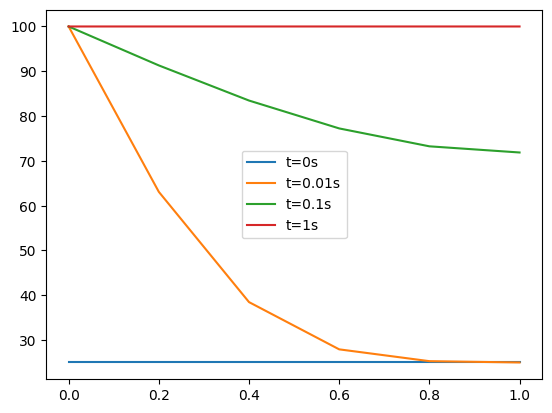
After running, plot your solution over \(x\) at time steps 0, 10, 100 and 999 together on the same plot
# run the solver
x,T = run_diffusion(L=1,
                      dx=0.1,
                      dt=0.001,
                      kappa=1,
                      T_init=25,
                      T_left=100,
                      h_right=0,
                      n_steps=1000
                     )

# plot the solution
plt.plot(x,T[0,:],label='t=0s')
plt.plot(x,T[10,:],label='t=0.01s')
plt.plot(x,T[100,:],label='t=0.1s')
plt.plot(x,T[-1,:],label='t=1s')
plt.legend();

See how even though the parameters can be neatly organized into the four logical groups above? Nevertheless, they all get jammed together in the same function call and the best we can do is to order them in some sensible way.
# run the solver
x,T = run_diffusion(L=1,
                      dx=0.1,
                      dt=0.001,
                      kappa=5,
                      T_init=25,
                      T_left=100,
                      h_right=0,
                      n_steps=1000
                     )

# plot the solution
plt.plot(x,T[0,:],label='t=0s')
plt.plot(x,T[10,:],label='t=0.01s')
plt.plot(x,T[100,:],label='t=0.1s')
plt.plot(x,T[-1,:],label='t=1s')
plt.legend();

Did you notice how to change only one parameter you had to repeat all the others? This is common in the functional programming paradigm: without global variables, functions calls tend to involve a large number of arguments and make the code look a bit clunky. It also involves a risk: maybe when copy/pasting you change some other parameter by mistake that you did not want to touch.
Also notice how you had to do the plotting manually again. You could have implemented a dedicated plotting function, but even then you would need to keep passing x and T between functions. Not very clean.
Extending the solver#
For the final task of this part, the goal is to code a modified version of the solver in which we do not apply a flux BC on the right but another fixed temperature \(T_\mathrm{right}\). One possible way to do this is to add an if statement in the original code, but the function would then need yet another argument to inform it that the BC is now a fixed temperature and not a flux, otherwise it would have no way to discern that just from the value of the argument. Instead let us just code the whole thing again with a different name.
def run_diffusion_two(
    L,       # length of the bar
    dx,      # discretization in space
    dt,      # discretization in time
    kappa,   # heat diffusivity
    T_init,  # initial temperature
    T_left,  # Temperature on the left
    T_right, # Temperature on the right
    n_steps, # number of time steps
):
    assert kappa*dt/dx/dx<=0.5, 'Stability condition not satisfied'

    # spatial discretization
    x = np.arange(0, L+dx, dx)
    nx = len(x)

    # solution vectors
    T = np.zeros((n_steps,nx))

    # temperature field at t=0
    T[0,:] = T_init

    # loop through time
    for n in range(n_steps-1):
        # solution on the left
        T[n+1,0] = T_left

        # solution in the interior
        for m in range(1,nx-1):
            T[n+1,m] = T[n,m] + kappa*dt/dx/dx * (T[n,m+1]-2*T[n,m]+T[n,m-1])

        # solution on the right
        T[n+1,-1] = T_right

    return x, T
Let us now try it out.
Run the new solver with the same parameter set of the first example (\(\kappa=1\)) but now with \(T_\mathrm{right}=50\)
# run the solver
x,T = run_diffusion_two(L=1,
                      dx=0.1,
                      dt=0.001,
                      kappa=1,
                      T_init=25,
                      T_left=100,
                      T_right=50,
                      n_steps=1000
                     )

# plot the solution
plt.plot(x,T[0,:],label='t=0s')
plt.plot(x,T[10,:],label='t=0.01s')
plt.plot(x,T[100,:],label='t=0.1s')
plt.plot(x,T[-1,:],label='t=1s')
plt.legend();

Notice how much code we had to repeat in order to make such a small change. This is another drawback of functional programming: extending existing code often involves either a lot of repeated code or a convoluted set of if-then-else statements coupled with even more function arguments.
By Iuri Rocha and Marcel Zijlema, Delft University of Technology. CC BY 4.0, more info on the Credits page of Workbook.
