
Assignment#
Part 1: Introduction and set up#
In this assignment, you will investigate the joint variability of three soil properties. Soil properties vary naturally from sample to sample due to differences in soil composition, depositional history, stress history, and water content. These properties may also be statistically dependent. Therefore, considering them jointly can provide information that is not captured when each property is analysed separately.
The dataset Soil Properties contains laboratory soil-characterisation data. In this exercise, we focus on three random variables:
Unit weight, \(\gamma\) (\(\mathrm{kN/m^3}\))
Water content, \(w\) (%)
Plasticity index, \(PI\) (%)
import numpy as np
from scipy.stats import multivariate_normal
from scipy.stats import norm
import matplotlib.pyplot as plt
from statistics import mean, stdev
import os
from urllib.request import urlretrieve

def findfile(fname):
    if not os.path.isfile(fname):
        print(f'Downloading {fname}...')
        urlretrieve('https://github.com/TUDelft-MUDE/source-files/raw/main/file/'+fname, fname)

fname = 'Soil_Properties.csv'
findfile(fname)
Downloading Soil_Properties.csv...
# Load the three soil-property columns from the input file
raw = np.genfromtxt(fname, delimiter=',', names=True, dtype=float, encoding=None)

gamma = np.asarray(raw['gamma'], dtype=float)
w = np.asarray(raw['w'], dtype=float)
PI = np.asarray(raw['PI'], dtype=float)

data = np.column_stack((gamma, w, PI))

print(f'Number of complete observations = {len(data)}')
data
Number of complete observations = 127
array([[ 15.2       ,  74.4       ,  20.4       ],
       [ 14.9       ,  78.4       ,  34.2       ],
       [ 14.86250955,  44.42056396,  26.2       ],
       [ 14.99187335,  69.94963626,  33.5       ],
       [ 14.90279298,  70.70049394,  30.1       ],
       [ 17.5       ,  51.5       ,  16.5       ],
       [ 18.1       ,  39.4       ,  18.4       ],
       [ 16.1       ,  53.4       ,  18.4       ],
       [ 17.        ,  50.4       ,  26.9       ],
       [ 17.        ,  46.8       ,  29.3       ],
       [ 18.8       ,  32.9       ,  16.8       ],
       [ 16.8       ,  57.3       ,  27.6       ],
       [ 15.4069588 ,  66.72077922,  31.7       ],
       [ 15.8       ,  68.1       ,  30.2       ],
       [ 15.99356031,  64.40009855,  26.7       ],
       [ 15.8       ,  53.4       ,  22.7       ],
       [ 14.59817549,  69.5545766 ,  36.4       ],
       [ 14.2       ,  88.6       ,  51.3       ],
       [ 17.7       ,  32.2       ,  26.        ],
       [ 14.9       ,  69.1       ,  12.1       ],
       [ 14.5       ,  84.3       ,  35.5       ],
       [ 14.6       ,  83.9       ,  23.6       ],
       [ 14.2       ,  98.9       ,  30.6       ],
       [ 14.9       ,  72.3       ,  35.9       ],
       [ 11.4       , 208.4       , 116.9       ],
       [ 15.6       ,  69.1       ,  46.2       ],
       [ 15.        ,  75.        ,  49.8       ],
       [ 15.        ,  78.5       ,  45.1       ],
       [ 14.6       ,  83.1       ,  48.5       ],
       [ 18.        ,  39.9       ,  28.9       ],
       [ 17.        ,  47.4       ,  33.4       ],
       [ 17.2       ,  47.3       ,  32.        ],
       [ 14.4       ,  84.8       ,  53.2       ],
       [ 14.8       ,  73.        ,  49.5       ],
       [ 16.4       ,  51.7       ,  35.4       ],
       [ 15.8       ,  61.8       ,  37.7       ],
       [ 15.6       ,  59.2       ,  40.6       ],
       [ 15.5       ,  66.        ,  37.6       ],
       [ 16.4       ,  53.9       ,  24.3       ],
       [ 17.8       ,  39.9       ,  41.8       ],
       [ 16.4       ,  58.        ,  39.2       ],
       [ 15.6       ,  69.7       ,  28.7       ],
       [ 14.4       ,  85.6       ,  31.6       ],
       [ 15.9       ,  63.7       ,  33.6       ],
       [ 15.9       ,  63.4       ,  35.3       ],
       [ 18.        ,  39.8       ,  11.4       ],
       [ 17.26      ,  51.        ,  21.04      ],
       [ 12.17      , 209.3       ,  69.        ],
       [ 12.57      , 168.4       ,  57.        ],
       [ 17.5       ,  38.8       ,  53.1       ],
       [ 15.5       ,  69.7       ,  25.1       ],
       [ 16.1       ,  60.3       ,  26.7       ],
       [ 15.3       ,  73.4       ,  50.3       ],
       [ 14.9       ,  78.1       ,  41.7       ],
       [ 15.6       ,  67.8       ,  35.5       ],
       [ 14.8       ,  81.5       ,  57.41      ],
       [ 14.8       ,  78.6       ,  49.92      ],
       [ 15.2       ,  77.8       ,  62.05      ],
       [ 16.4       ,  58.1       ,  16.        ],
       [ 18.5       ,  35.1       ,   9.8       ],
       [ 16.3       ,  53.4       ,  45.83      ],
       [ 13.2       , 127.1       ,  77.96      ],
       [ 14.7       ,  82.7       ,  63.33      ],
       [ 13.5       , 110.4       ,  74.37      ],
       [ 16.4       ,  57.9       ,  28.2       ],
       [ 18.1       ,  36.9       ,   4.5       ],
       [ 13.4       , 137.2       ,  43.4       ],
       [ 13.4       , 130.        ,  71.61      ],
       [ 14.94998849,  78.60733113,  29.5       ],
       [ 14.89355021,  73.40501792,  28.5       ],
       [ 14.89947063,  79.94227994,  23.2       ],
       [ 13.9       , 113.9       ,  59.8       ],
       [ 15.14034063,  81.88818212,  40.1       ],
       [ 13.61621495, 102.6122449 ,  16.1       ],
       [ 17.5       ,  37.4       ,   7.8       ],
       [ 18.3       ,  37.5       ,  45.8       ],
       [ 18.        ,  44.1       ,  15.9       ],
       [ 16.8       ,  41.7       ,  37.9       ],
       [ 16.9       ,  47.2       ,  15.8       ],
       [ 17.        ,  43.1       ,  18.        ],
       [ 15.1575753 ,  60.38031939,  21.6       ],
       [ 12.6       , 119.4       ,  22.8       ],
       [ 13.8       , 126.5       ,  44.6       ],
       [ 14.2       ,  19.        ,  16.        ],
       [ 13.6       ,  95.3       ,  49.6       ],
       [ 14.4       ,  89.3       ,  44.6       ],
       [ 13.        , 140.9       ,  40.3       ],
       [ 13.39023954, 119.3477895 ,  63.3       ],
       [ 16.36915481,  58.08145873,  32.8       ],
       [ 15.85069948,  64.64571781,  31.4       ],
       [ 15.85069948,  20.20692758,  66.2       ],
       [ 13.41292897,  82.1573132 ,  66.1       ],
       [ 15.82119038,  60.43704475,  29.7       ],
       [ 14.45333159,  91.42430008,  40.9       ],
       [ 14.6847641 ,  74.58860211,  19.1       ],
       [ 16.17296693,  62.74509804,  22.        ],
       [ 15.34300367,  60.18387553,  21.        ],
       [ 16.12082636,  52.00774069,  23.3       ],
       [ 11.12528692, 272.1070812 , 133.9       ],
       [ 12.23993361, 135.4605659 ,  69.5       ],
       [ 12.        , 147.1       ,  21.3       ],
       [ 14.24974457,  98.84481701,  37.9       ],
       [ 15.3       ,  80.4       ,   3.6       ],
       [ 15.2236069 ,  72.64197531,  37.9       ],
       [ 15.5       ,  74.4       ,  12.        ],
       [ 14.8078985 ,  53.21313374,  30.        ],
       [ 13.95462238,  98.17837365,  34.        ],
       [ 15.        ,  83.6       ,  50.44      ],
       [ 13.6       , 114.        ,  80.1       ],
       [ 10.8       , 306.8       ,  84.9       ],
       [ 12.6       , 136.5       ,  81.7       ],
       [ 14.        ,  97.8       ,  42.7       ],
       [ 14.7       ,  86.3       ,  57.2       ],
       [ 17.3       ,  40.1       ,  14.3       ],
       [ 16.7       ,  49.6       ,   7.8       ],
       [ 16.9       ,  42.2       ,  12.        ],
       [ 17.5       ,  42.6       ,  13.1       ],
       [ 16.21      ,  50.6       ,  24.        ],
       [ 15.5       ,  68.        ,  14.        ],
       [ 14.036148  ,  93.35135135,  53.6       ],
       [ 14.291208  ,  94.55128205,  54.9       ],
       [ 13.667292  ,  96.55756208,  71.9       ],
       [ 13.698684  , 121.6507937 ,  52.5       ],
       [ 15.083856  ,  72.99729973,  35.6       ],
       [ 14.346144  ,  92.92875989,  98.4       ],
       [ 14.561964  ,  90.40533607,  30.1       ],
       [ 13.836024  , 111.5176965 ,  33.8       ]])
Part 2: Data exploration#
Task 2.1:
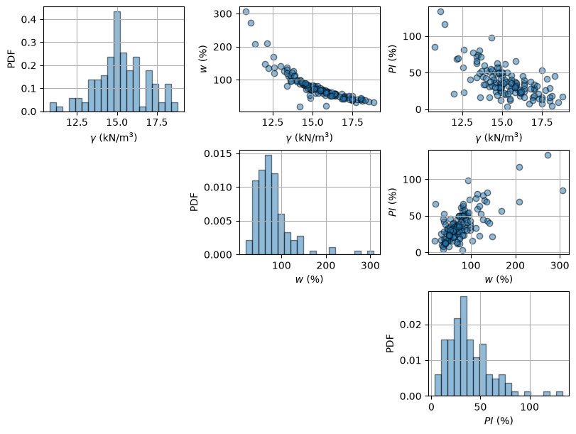
Plot the data. Examine the histogram of each soil property and the scatter plots for each pair of properties.
What can you conclude about:
the shape and variability of the marginal distributions; and
the direction and approximate strength of dependence between the soil properties?
variable_names = [
    r'$\gamma$ (kN/m$^3$)',
    r'$w$ (%)',
    r'$PI$ (%)'
]

fig, axs = plt.subplots(3, 3, figsize=(8, 6), layout='constrained')

for i in range(data.shape[1]):
    for j in range(data.shape[1]):
        if i == j:
            axs[i, j].grid()
            axs[i, j].hist(
                data[:, i],
                bins=20,
                density=True,
                alpha=0.5,
                edgecolor='black'
            )
            axs[i, j].set_xlabel(variable_names[i])
            axs[i, j].set_ylabel('PDF')

        elif i < j:
            axs[i, j].grid()
            axs[i, j].scatter(
                data[:, i],
                data[:, j],
                alpha=0.5,
                edgecolor='black'
            )

            axs[i, j].set_xlabel(variable_names[i])
            axs[i, j].set_ylabel(variable_names[j])

        else:
            axs[i, j].axis('off')
plt.show()
Solution 2.1:
The plots show considerable variability in the three soil properties and clear dependence between them.
The scatter plots indicate that:
\(\gamma\) and \(w\) have a strong negative relationship: soils with higher water content tend to have lower unit weight.
\(w\) and \(PI\) have a positive relationship: soils with higher water content tend to have a higher plasticity index.
\(\gamma\) and \(PI\) have a negative relationship: soils with higher plasticity index tend to have lower unit weight.
The marginal distributions also have different shapes. The distribution of \(\gamma\) is relatively concentrated and approximately bell-shaped, although some deviations from a Gaussian distribution are visible. In contrast, \(w\) and \(PI\) are clearly right-skewed, with most observations concentrated at lower values and a small number of much larger values.
Therefore, although the variables show clear dependence, the observed marginal distributions—particularly those of \(w\) and \(PI\)—are not well described by Gaussian distributions.
Task 2.2:
Quantify the strength of the linear dependence between each pair using Pearson’s correlation coefficient. What can you conclude?
Solution 2.2:
As expected from the first observation of the data, we can see that \(\gamma\) and \(w\) are strongly negatively correlated with a correlation of -0.85, while \(\gamma\) and \(PI\) are negatively correlated with a correlation of -0.64. In contrast, \(w\) and \(PI\) are positively correlated with a correlation of 0.68.
This means that soils with a higher water content (\(w\)) tend to have a lower unit weight (\(\gamma\)) and a higher plasticity index (\(PI\)). Similarly, soils with a higher plasticity index tend to have a lower unit weight.
def calculate_covariance(X1, X2):
    mean_x1 = mean(X1)
    mean_x2 = mean(X2)

    diff_x1 = X1- mean_x1
    diff_x2 = X2- mean_x2

    product = diff_x1*diff_x2

    # Sample covariance: divide by n - 1
    covariance = sum(product) / (len(product) - 1)

    return covariance

def pearson_correlation(X1, X2):
    covariance = calculate_covariance(X1, X2)
    correl_coeff = covariance / (stdev(X1) * stdev(X2))

    return correl_coeff

print("Pearson's correlation coefficient between γ and w is",
      np.round(pearson_correlation(data[:,0], data[:,1]), 3))

print("Pearson's correlation coefficient between γ and PI is",
      np.round(pearson_correlation(data[:,0], data[:,2]), 3))

print("Pearson's correlation coefficient between w and PI is",
      np.round(pearson_correlation(data[:,1], data[:,2]), 3))
Pearson's correlation coefficient between γ and w is -0.849
Pearson's correlation coefficient between γ and PI is -0.642
Pearson's correlation coefficient between w and PI is 0.684
Part 3: Multivariate Gaussian distribution#
Task 3.1:
Model the joint distribution of \(\gamma\), \(w\) and \(PI\) using a multivariate Gaussian distribution. Follow the steps:
Define the vector of means.
Define the covariance matrix.
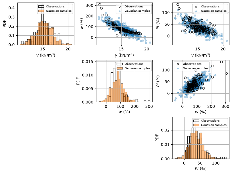
Draw 500 samples from the fitted trivariate Gaussian distribution and compare them with the observations.
Do you see differences between the observations and the Gaussian samples? Compare both the univariate marginal distributions and the bivariate scatter plots.
Solution 3.1:
Overall, the fitted multivariate Gaussian distribution provides a reasonable approximation to the observed soil-property data. The Gaussian samples reproduce the general range and concentration of most observations and capture the main dependence between the variables: a negative relationship between \(\gamma\) and \(w\), a negative relationship between \(\gamma\) and \(PI\), and a positive relationship between \(w\) and \(PI\).
The marginal distributions of the Gaussian samples also agree reasonably well with the main body of the observations. However, the observed data contain some extreme values and longer tails, particularly for \(w\) and \(PI\), which are not well reproduced by the fitted Gaussian distribution.
Therefore, the multivariate Gaussian distribution can be considered a useful approximation for describing the general variability and dependence of the soil properties, although it may not adequately represent the extreme observations and tail behaviour.
# ---------------------------------------------------------
# Define the vector of means
# ---------------------------------------------------------
mu1 = mean(data[:, 0])
mu2 = mean(data[:, 1])
mu3 = mean(data[:, 2])

mu = [mu1, mu2, mu3]

# ---------------------------------------------------------
# Define the covariance matrix
# ---------------------------------------------------------
s1 = stdev(data[:, 0])
s2 = stdev(data[:, 1])
s3 = stdev(data[:, 2])

covariance_12 = calculate_covariance(data[:, 0], data[:, 1])
covariance_13 = calculate_covariance(data[:, 0], data[:, 2])
covariance_23 = calculate_covariance(data[:, 1], data[:, 2])

sigma = np.array([
    [s1**2,        covariance_12, covariance_13],
    [covariance_12, s2**2,       covariance_23],
    [covariance_13, covariance_23, s3**2]
])

# ---------------------------------------------------------
# Draw 500 samples from the fitted trivariate Gaussian
# ---------------------------------------------------------
samples = multivariate_normal(
    mean=mu,
    cov=sigma
).rvs(size=500)

# ---------------------------------------------------------
# Compare samples with observations
# ---------------------------------------------------------
fig, axs = plt.subplots(
    3, 3,
    figsize=(8, 6),
    layout='constrained'
)

for i in range(data.shape[1]):
    for j in range(data.shape[1]):
        # Marginal distributions
        if i == j:
            axs[i, j].grid()
            axs[i, j].hist(
                data[:, i],
                bins=20,
                density=True,
                alpha=0.9,
                edgecolor='black',
                facecolor='none',
                label='Observations'
            )

            axs[i, j].hist(
                samples[:, i],
                bins=20,
                density=True,
                alpha=0.5,
                edgecolor='black',
                label='Gaussian samples'
            )

            axs[i, j].set_xlabel(variable_names[i])
            axs[i, j].set_ylabel('PDF')

            axs[i, j].legend(fontsize=7)

        # Scatter plots
        elif i < j:
            axs[i, j].grid()
            # Gaussian samples first
            axs[i, j].scatter(
                samples[:, i],
                samples[:, j],
                alpha=0.30,
                s=20,
                label='Gaussian samples'
            )
            # Observations on top
            axs[i, j].scatter(
                data[:, i],
                data[:, j],
                alpha=0.9,
                s=30,
                edgecolor='black',
                facecolor='none',
                label='Observations'
            )

            axs[i, j].set_xlabel(variable_names[i])
            axs[i, j].set_ylabel(variable_names[j])

            # Put observations first in legend
            handles, labels = axs[i, j].get_legend_handles_labels()

            axs[i, j].legend(
                [handles[1], handles[0]],
                [labels[1], labels[0]],
                fontsize=7,
                markerscale=0.7
            )

        else:
            axs[i, j].axis('off')

plt.show()
Task 3.2:
Suppose we are interested in soil with the following properties:
unit weight: \(\gamma < 16\ \mathrm{kN/m^3}\)
water content: \(w > 80\%\)
plasticity index: \(PI > 30\%\)
Using samples generated from the fitted multivariate Gaussian distribution, estimate the probability that all three conditions are satisfied at the same time.
Repeat the calculation using different numbers of samples,
\[ >N = 100,\quad 1{,}000,\quad 10{,}000,\quad 100{,}000,\quad 1{,}000{,}000. >\]How does the estimated probability behave as the number of samples increases? Comment on the stability of the estimate.
Hint: For each generated sample, check whether all three conditions are satisfied. The probability can be estimated as the proportion of generated samples that satisfy all three conditions.
Solution 3.2:
For small sample sizes, the estimated probability can vary considerably. As \(N\) increases, the estimate becomes more stable and converges towards approximately \(0.41\). Therefore, using more samples gives a more reliable estimate of the probability.
# Investigate the effect of sample size
sample_sizes = [100, 1_000, 10_000, 100_000, 1_000_000]

for N in sample_sizes:

    # Draw samples from the fitted multivariate Gaussian distribution
    samples = multivariate_normal(mean=mu, cov=sigma).rvs(size=N)

    # Check the three screening criteria simultaneously
    condition = (
        (samples[:, 0] < 16) &
        (samples[:, 1] > 80) &
        (samples[:, 2] > 30)
    )

    # Estimate the probability
    prob_meeting_condition = np.mean(condition)

    print(f'N = {N:9d}: estimated probability = {prob_meeting_condition:.4f}')
    print(f'N = {N:6d}: estimated probability = {prob_meeting_condition:.4f}')
N =       100: estimated probability = 0.3400
N =    100: estimated probability = 0.3400
N =      1000: estimated probability = 0.4140
N =   1000: estimated probability = 0.4140
N =     10000: estimated probability = 0.4085
N =  10000: estimated probability = 0.4085
N =    100000: estimated probability = 0.4111
N = 100000: estimated probability = 0.4111
N =   1000000: estimated probability = 0.4099
N = 1000000: estimated probability = 0.4099
Part 4: Conditioning the multivariate Gaussian distribution#
Task 4.1:
Suppose a laboratory measurement gives a water content of
\[ >w = 120\% >\]which is above the sample mean. What does this observation imply for the joint distribution of unit weight \(\gamma\) and plasticity index \(PI\)?
Compute the conditional distribution of \(\gamma\) and \(PI\) given \(w = 120\%\).
Compute the conditional probability
\[ >P\left( >\gamma < 16\ \mathrm{kN/m^3}, >\quad >PI > 30\% >\mid >w = 120\% >\right). >\]
Solution 4.1:
For a multivariate Gaussian distribution, conditioning on one variable gives another Gaussian distribution. Here, we condition on \(w\) and obtain a bivariate Gaussian distribution for \(\gamma\) and \(PI\).
For \(w = 120\%\), the conditional mean vector is
\[\begin{split} >\boldsymbol{\mu}_{X\mid w=120} >= >\begin{bmatrix} >13.922 \\ >52.470 >\end{bmatrix}, >\end{split}\]where \(X=[\gamma,PI]^T\). Therefore,
\[ >E[\gamma\mid w=120\%] = 13.922\ \mathrm{kN/m^3}, >\]and
\[ >E[PI\mid w=120\%] = 52.470\%. >\]The conditional covariance matrix is
\[\begin{split} >\boldsymbol{\Sigma}_{X\mid w=120} >= >\begin{bmatrix} >0.715 & -2.131 \\ >-2.131 & 251.538 >\end{bmatrix}. >\end{split}\]Since \(w=120\%\) is higher than its sample mean of \(78.946\%\), the conditional results are consistent with the observed correlations. Because \(w\) and \(\gamma\) are strongly negatively correlated, a high value of \(w\) is associated with a lower expected unit weight. In contrast, because \(w\) and \(PI\) are positively correlated, a high value of \(w\) is associated with a higher expected plasticity index.
Using samples generated from this conditional Gaussian distribution, the estimated probability is
\[ >P\left( >\gamma < 16\ \mathrm{kN/m^3}, >\quad >PI > 30\% >\mid >w=120\% >\right) >\approx 0.917. >\]Thus, according to the fitted Gaussian model, given a water content of \(120\%\), there is approximately a 91.7% probability that the unit weight is below \(16\ \mathrm{kN/m^3}\) and the plasticity index is above \(30\%\) simultaneously.
# Conditional distribution of X = [γ, PI] given Y = w = 120%

a = 120.0

# Partition the mean vector for X = [gamma, PI] and Y = w
mu_X = np.array([
    mu[0],      # mean of gamma
    mu[2]       # mean of PI
])

mu_Y = mu[1]    # mean of w

# Partition the covariance matrix
Sigma_XX = np.array([
    [sigma[0, 0], sigma[0, 2]],
    [sigma[2, 0], sigma[2, 2]]
])

Sigma_XY = np.array([
    [sigma[0, 1]],
    [sigma[2, 1]]
])

Sigma_YY = sigma[1, 1]

# ---------------------------------------------------------
# Conditional Gaussian equations
#
# mu_X|Y = mu_X + Sigma_XY * Sigma_YY^(-1) * (a - mu_Y)
#
# Sigma_X|Y = Sigma_XX
#             - Sigma_XY * Sigma_YY^(-1) * Sigma_YX
# ---------------------------------------------------------

# Conditional mean vector
cond_mu_vector = (
    mu_X
    + (Sigma_XY[:, 0] / Sigma_YY) * (a - mu_Y)
)

# Conditional covariance matrix
cond_sigma_matrix = (
    Sigma_XX
    - (Sigma_XY @ Sigma_XY.T) / Sigma_YY
)

# Conditional standard deviations
cond_std = np.sqrt(np.diag(cond_sigma_matrix))

print('Conditional mean [γ, PI] =')
print(np.round(cond_mu_vector, 3))

print('\nConditional covariance matrix =')
print(np.round(cond_sigma_matrix, 3))

print('\nConditional standard deviations [γ, PI] =')
print(np.round(cond_std, 3))

# ---------------------------------------------------------
# Generate samples from the conditional Gaussian distribution
# ---------------------------------------------------------
N = 100000

cond_samples = multivariate_normal(
    mean=cond_mu_vector,
    cov=cond_sigma_matrix
).rvs(size=N)

# ---------------------------------------------------------
# Estimate P(gamma < 16, PI > 30 | w = 120%)
# ---------------------------------------------------------
condition = (
    (cond_samples[:, 0] < 16) &
    (cond_samples[:, 1] > 30)
)

cond_prob = np.mean(condition)
print(
    f'\nConditional probability '
    f'P(γ < 16, PI > 30 | w = 120%) = {cond_prob:.4f}'
)
Conditional mean [γ, PI] =
[13.922 52.47 ]

Conditional covariance matrix =
[[  0.715  -2.131]
 [ -2.131 251.538]]

Conditional standard deviations [γ, PI] =
[ 0.846 15.86 ]

Conditional probability P(γ < 16, PI > 30 | w = 120%) = 0.9164
Task 4.2:
Using the results from the previous task, compare the conditional and unconditional distributions of \(\gamma\) and \(PI\).
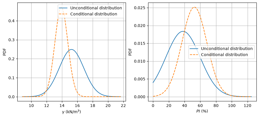
Plot the conditional and unconditional marginal distributions of \(\gamma\) and \(PI\).
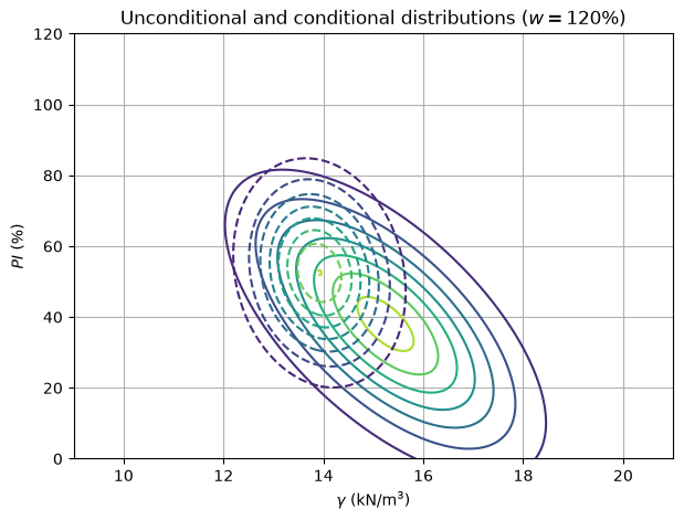
Plot the conditional and unconditional joint probability density contours of \(\gamma\) and \(PI\).
Compare the two cases and explain:
how the mean values change after conditioning on \(w = 120\%\);
how the uncertainty changes;
how these changes are related to the correlations of \(\gamma\) and \(PI\) with \(w\).
Solution 4.2a:
The observed value \(w = 120\%\) is above the mean water content.
Since \(\gamma\) and \(w\) have a strong negative correlation,
\[ >\rho_{\gamma,w} = -0.8495, >\]conditioning on a relatively high value of \(w\) shifts the distribution of \(\gamma\) toward lower values. The conditional distribution is also substantially narrower than the unconditional distribution, indicating that observing \(w\) considerably reduces the uncertainty in \(\gamma\).
In contrast, \(PI\) and \(w\) are positively correlated,
\[ >\rho_{w,PI} = 0.6837. >\]Therefore, conditioning on \(w = 120\%\) shifts the distribution of \(PI\) toward higher values. Its conditional distribution is also narrower, showing that the observed value of \(w\) provides additional information about \(PI\).
The reduction in uncertainty is more pronounced for \(\gamma\) than for \(PI\), which is consistent with the stronger absolute correlation between \(\gamma\) and \(w\).
# Compare conditional and unconditional marginals of γ and PI

# γ
values_gamma = np.linspace(
    max(0, mu[0] - 4*np.sqrt(sigma[0,0])),
    mu[0] + 4*np.sqrt(sigma[0,0]),
    200
)

uncond_γ_pdf = norm.pdf(
    values_gamma,
    loc=mu[0],
    scale=np.sqrt(sigma[0,0])
)

cond_γ_pdf = norm.pdf(
    values_gamma,
    loc=cond_mu_vector[0],
    scale=np.sqrt(cond_sigma_matrix[0,0])
)

# PI
values_PI = np.linspace(
    max(0, mu[2] - 4*np.sqrt(sigma[2,2])),
    mu[2] + 4*np.sqrt(sigma[2,2]),
    200
)

uncond_PI_pdf = norm.pdf(
    values_PI,
    loc=mu[2],
    scale=np.sqrt(sigma[2,2])
)

cond_PI_pdf = norm.pdf(
    values_PI,
    loc=cond_mu_vector[1],
    scale=np.sqrt(cond_sigma_matrix[1,1])
)

# Plot marginal distributions
fig, ax = plt.subplots(1, 2, figsize=(9, 4), layout='constrained')

# γ
ax[0].plot(
    values_gamma,
    uncond_γ_pdf,
    label='Unconditional distribution'
)

ax[0].plot(
    values_gamma,
    cond_γ_pdf,
    '--',
    label='Conditional distribution'
)

ax[0].grid()
ax[0].set_xlabel(r'$\gamma$ (kN/m$^3$)')
ax[0].set_ylabel('PDF')
ax[0].legend()

# PI
ax[1].plot(
    values_PI,
    uncond_PI_pdf,
    label='Unconditional distribution'
)

ax[1].plot(
    values_PI,
    cond_PI_pdf,
    '--',
    label='Conditional distribution'
)

ax[1].grid()
ax[1].set_xlabel(r'$PI$ (%)')
ax[1].set_ylabel('PDF')
ax[1].legend()

plt.show()
Solution 4.2b:
The joint probability density contours show the same general effect as the marginal distributions. Conditioning on \(w = 120\%\) shifts the centre of the joint \((\gamma, PI)\) distribution toward lower \(\gamma\) and higher \(PI\).
The conditional contours are also more concentrated than the unconditional contours, indicating a reduction in uncertainty once \(w\) is known. This is consistent with the narrower conditional marginal distributions observed previously.
The shape and orientation of the contours also change after conditioning. This shows that observing \(w\) affects not only the individual uncertainties in \(\gamma\) and \(PI\), but also their joint dependence.
Overall, knowing the water content provides additional information about both soil properties and results in a more concentrated joint distribution.
# Compare joint conditional and unconditional distributions of γ and PI

# ---------------------------------------------------------
# 1. Create values for γ and PI
# ---------------------------------------------------------

values_gamma = np.linspace(9, 21, 200)
values_PI = np.linspace(0, 120, 200)

# Create a two-dimensional grid of γ and PI
G, I = np.meshgrid(values_gamma, values_PI)

# ---------------------------------------------------------
# 2. Define the unconditional distribution of [γ, PI]
# ---------------------------------------------------------

uncond_mu = [
    mu[0],      # mean of γ
    mu[2]       # mean of PI
]

uncond_cov = np.array([
    [sigma[0, 0], sigma[0, 2]],
    [sigma[2, 0], sigma[2, 2]]
])

# ---------------------------------------------------------
# 3. Calculate the joint PDFs
# ---------------------------------------------------------

# Create pairs of [γ, PI] values
X = np.array([
    np.concatenate(G.T),
    np.concatenate(I.T)
]).T

# Unconditional joint PDF
Z_uncond = multivariate_normal(
    mean=uncond_mu,
    cov=uncond_cov
).pdf(X)

# Conditional joint PDF given w = 120%
Z_cond = multivariate_normal(
    mean=cond_mu_vector,
    cov=cond_sigma_matrix
).pdf(X)

# Convert the PDF values back to the two-dimensional grid
Z_uncond = Z_uncond.reshape(G.T.shape).T
Z_cond = Z_cond.reshape(G.T.shape).T

# ---------------------------------------------------------
# 4. Plot the contours
# ---------------------------------------------------------

fig, ax = plt.subplots(figsize=(7, 5))

ax.contour(
    G, I, Z_uncond,
    levels=8,
    linestyles='-'
)

ax.contour(
    G, I, Z_cond,
    levels=8,
    linestyles='--'
)

ax.grid()

ax.set_xlabel(r'$\gamma$ (kN/m$^3$)')
ax.set_ylabel(r'$PI$ (%)')
ax.set_title(
    r'Unconditional and conditional distributions ($w=120\%$)'
)

plt.show()
Solution 4.2c:
Conditioning on \(w=120\%\) changes both the mean values and the uncertainty of \(\gamma\) and \(PI\).
The mean unit weight decreases from
\[ >\mu_{\gamma}=15.243 >\quad \text{to} \quad >\mu_{\gamma\mid w=120}=13.922\ \mathrm{kN/m^3}. >\]This is consistent with the strong negative correlation between \(\gamma\) and \(w\) (\(\rho_{\gamma,w}=-0.8495\)): a higher water content is associated with a lower unit weight.
In contrast, the mean plasticity index increases from
\[ >\mu_{PI}=38.050\% >\quad \text{to} \quad >\mu_{PI\mid w=120}=52.470\%. >\]This is consistent with the positive correlation between \(PI\) and \(w\) (\(\rho_{w,PI}=0.6837\)): a higher water content is associated with a higher plasticity index.
The conditional distributions are also narrower than the unconditional distributions. Once \(w\) is known, some of the uncertainty in \(\gamma\) and \(PI\) is reduced because both variables are correlated with \(w\).
Therefore, conditioning on a high water content shifts \(\gamma\) toward lower values, shifts \(PI\) toward higher values, and reduces the uncertainty in both variables.
By Zheng Guan, Delft University of Technology. CC BY 4.0, more info on the Credits page of Workbook.