
Part 2: Numerical solution of a linear ODE#
Reservoir storage and discharge#

As a measure to cope with climate change, the municipality of a metropolis considers the construction of a big underground reservoir collecting rainwater for a part of the city as a buffer in periods of heavy rain, to prevent urban flooding. Above the minimum water level \(h_{min}\), which acts as a reserve for the fire brigade to intake water for fire extinction, water can outflow the reservoir into the sewage system with reduced capacity. As a simplification, this outflow discharge is assumed proportional to the water level above the minimum level. Hence, the water level in the reservoir depends on both precipitation and discharge, while the latter is zero below the minimum level. If it rains heavily, the reservoir is filled up (\(h\) will increase) and in case of little or no rain, the reservoir will empty (\(h\) will decrease) down to the minimum level. The simplified system can be described by the following ordinary differential equation (ODE):
where:
\(h\) is the water level in the reservoir \(t\) is the time \(A_R\) is the storage area of the reservoir \(A\) is the total area above ground from which precipitation is collected \(P(t)\) is the precipitation (measured on frequent regular time intervals in \(mm/hour\)) \(K\) is a term that defines the proportionality of the discharge with respect to the water level in \(m^2/hour\)All areas are defined in \(m^2\), while \(h\) is defined in \(m\) and \(t\) in \(hour\).
The maximum reservoir depth is 20 m. The idea is to design the size (base area) of the reservoir (\(A_R\)) based on a design precipitation scheme of 200 mm in 48 hours, using an initial estimate of 7000 \(m^2\) (the size of a football field).
Task 2.1
Run the cells below to visualise the precipitation in the considered 48 hour time frame:
import matplotlib.pyplot as plt
%config InlineBackend.figure_formats = ['svg']
import numpy as np
AR = 7000       # Reservoir's base area
A  = 1000000    # Precipitation collection area (1 km^2)
K  = 200        # Discharge factor
h_min = 2.0     # Minimum reservoir level

hours = 48
t_data = np.arange(1, hours + 1)

P_data = np.array([0, 10, 0, 5, 30, 0, 0, 4, 2, 0, 0, 0, 80, 0, 0, 0, 0, 0, 14, 0, 3, 3, 0,
             0, 1, 4, 0, 0, 0, 0, 0, 0, 0, 10, 34, 0, 0, 0, 0, 0, 0, 0, 0, 0, 0, 0, 0, 0])

plt.bar(t_data, P_data)
plt.show()

print(f'Total discharge in 48 hours: {np.sum(P_data)} mm')
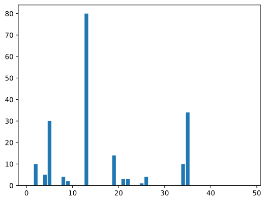
Total discharge in 48 hours: 200 mm
(Alternatively, read an input file with precipitation data)
Task 2.2
Formulate the Forward Euler scheme for the above ODE and elaborate this into an expression for \(h\) at the next time step (\(h_{i+1}\)).
Solution 2.2
\[ A_R \frac{h_{i+1} - h_i}{\Delta t} = \frac{A}{1000} P(t_i) - K \left(h_i - h_{min} \right) \]\[ h_{i+1} - h_i = \frac{\Delta t}{A_R} \left( \frac{A}{1000} P(t_i) - K \left(h_i - h_{min} \right) \right) \]\[ h_{i+1} = h_i + \frac{\Delta t}{A_R} \left( \frac{A}{1000} P(t_i) - K \left(h_i - h_{min} \right) \right) \]
Task 2.3
Complete and run the code cells below to calculate \(h_{i+1}\) for all time steps until the end of the time interval, considering \(h_0 = h_{min}\).
Data initialisation#
# Define the time step and create solution time points
dt = 0.1        # 0.1 hours = 6 minutes
num = int(hours / dt)
print(f"Number of time steps: {num}")
t = np.linspace(0, hours, num+1)

# Interpolate precipitation data to solution time points
indices = np.searchsorted(t_data, t, side='left')
P = P_data[indices]

assert len(P) == len(t)
Number of time steps: 480
Forward Euler scheme#
h = np.zeros_like(t)

h[0] = h_min

for i in range(num):
    h[i+1] = h[i] + dt/AR * (A/1000 * P[i] - K * (h[i] - h_min))
Task 2.4
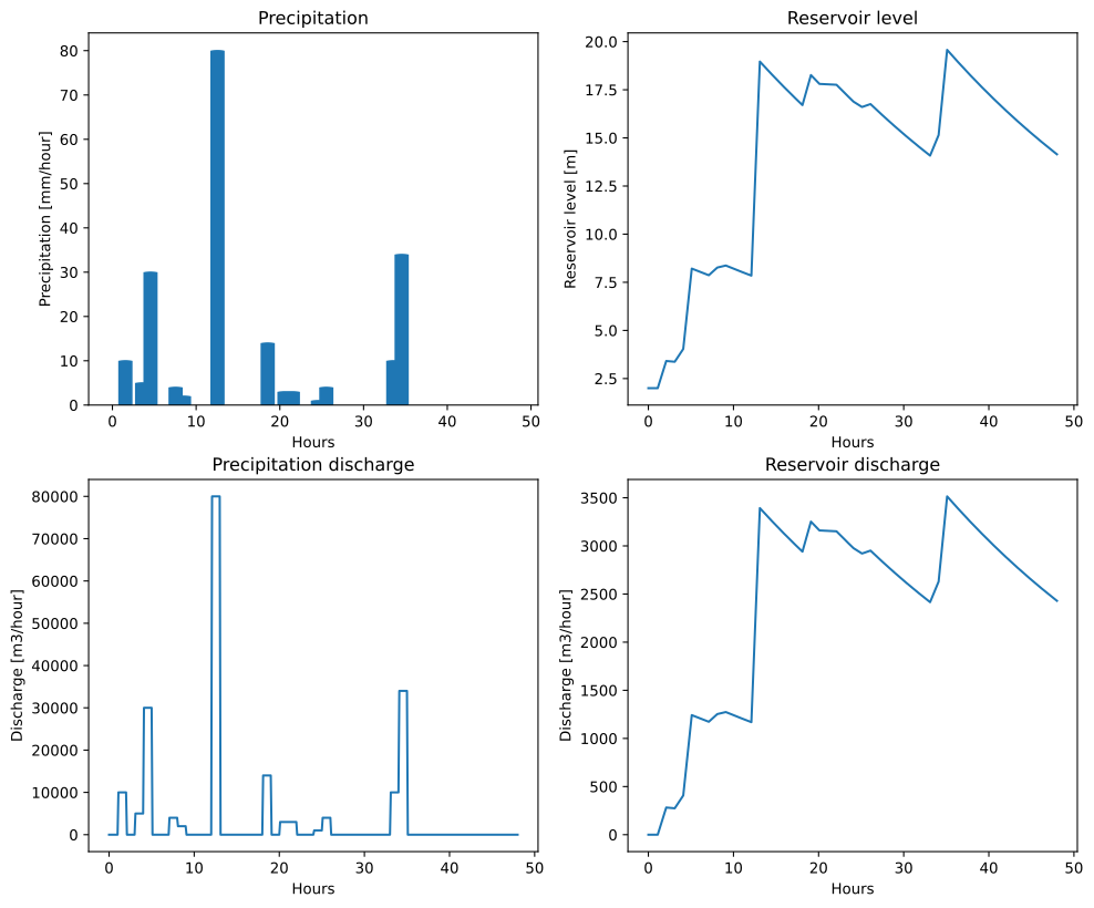
Run the code cell below to plot the results
def plot_figs():
    fig, ax = plt.subplots(nrows=2, ncols=2, figsize=(12, 10))

    ax[0,0].bar(t, P, label='Precipitation')
    ax[0,0].set_xlabel('Hours')
    ax[0,0].set_ylabel('Precipitation [mm/hour]')
    ax[0,0].set_title('Precipitation')

    ax[0,1].plot(t, h, label='Reservoir level')
    ax[0,1].set_xlabel('Hours')
    ax[0,1].set_ylabel('Reservoir level [m]')
    ax[0,1].set_title('Reservoir level')

    ax[1,0].plot(t, P*A/1000, label='Precipitation discharge')
    ax[1,0].set_xlabel('Hours')
    ax[1,0].set_ylabel('Discharge [m3/hour]')
    ax[1,0].set_title('Precipitation discharge')

    ax[1,1].plot(t, K*(h-h_min), label='Reservoir discharge')
    ax[1,1].set_xlabel('Hours')
    ax[1,1].set_ylabel('Discharge [m3/hour]')
    ax[1,1].set_title('Reservoir discharge')

plot_figs()
Task 2.5
Write a function (print_max()) to print the maximum values of:
The reservoir level
The maximum discharge flowing into the reservoir according to the design precipitation scheme
The maximum discharge from the reservoir
def print_max():
    print(f'Maximum reservoir level         : {np.max(h):.2f} m')
    print(f'Maximum precipitation discharge : {np.max(P*A/1000):.0f} m3/hour')
    print(f'Maximum reservoir discharge     : {np.max(K*(h-h_min)):.0f} m3/hour')

print_max()
Maximum reservoir level         : 19.57 m
Maximum precipitation discharge : 80000 m3/hour
Maximum reservoir discharge     : 3514 m3/hour
Task 2.6
Verify (analytically) the stability of the Forward Euler solution. Give the expression for the condition of stability.
Solution 2.6
We can reformulate the Forward Euler solution as:
\[ h_{i+1} = h_i \left( 1 - \frac{\Delta t K}{A_R} \right) + \frac{\Delta t}{A_R} \frac{A}{1000} P(t_i) + \frac{\Delta t K}{A_R} h_{min} \]The Forward Euler solution is stable if:
\[ \Delta t < 2 \frac{A_R}{K} \]Hence, \(\Delta t\) must be less than (2*7000 m²) / (200 m²/h) = 70 hour, while it is 0.1 hour, so perfectly fine! (However, note that with a time step of 70 hours, you would miss the dynamics in the precipitation signal. So even though the solution would be numerically stable, it would be incorrect.)
Task 2.7
Formulate the Backward (Implicit) Euler scheme for the above ODE and elaborate this into an expression for \(h\) at the next time step (\(h_{i+1}\)).
Hints:
Refer to next week’s lecture or Section 1.2 in the book for an application of the Backward Euler scheme:
It may be useful to introduce \(h^*\) as an offset to \(h\) considering \(h_{min}\):
\[h^* = h - h_{min} \]
Solution 2.7
Introducing \(h^*\) as an offset to \(h\) considering \(h_{min}\):
\[h^* = h - h_{min} \]while
\[ \frac{\partial h}{\partial t} = \frac{\partial h^*}{\partial t} \]With this:
\[ A_R \frac{h^*_{i+1} - h^*_i}{\Delta t} = \frac{A}{1000} P(t_{i+1}) - K h^*_{i+1} \]\[ \frac{A_R}{\Delta t} h^*_{i+1} + K h^*_{i+1} = \frac{A_R}{\Delta t} h^*_i + \frac{A}{1000} P(t_{i+1}) \]\[ h^*_{i+1} \left(\frac{A_R}{\Delta t} + K \right) = \frac{A_R}{\Delta t} h^*_i + \frac{A}{1000} P(t_{i+1}) \]\[ h^*_{i+1} = \frac{ \frac{A_R}{\Delta t} h^*_i + \frac{A}{1000} P(t_{i+1}) } {\left(\frac{A_R}{\Delta t} + K \right)} \]and \(h^*_0 = 0\)
The solution for \(h^*\) can be easily back transformed to \(h\) by:
\[ h = h_{min} + h^* \]
Task 2.8
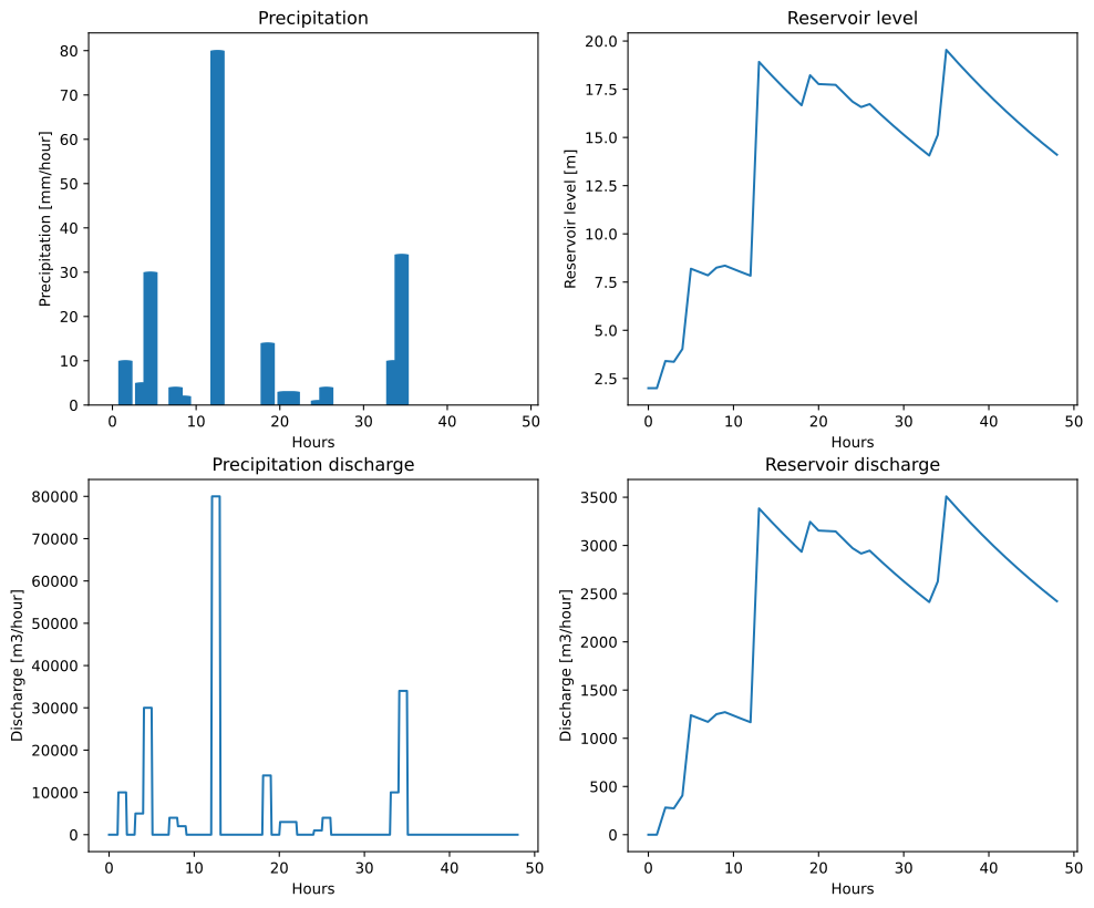
Complete and run the code cell below to calculate \(h_{i+1}\) for all time steps until the end of the time interval using the Backward Euler scheme.
Backward Euler scheme#
h_star = np.zeros_like(t)

h_star[0] = 0

for i in range(num):
    h_star[i+1] = (AR/dt * h_star[i] + A/1000 * P[i+1]) / (AR/dt + K)

h = h_min + h_star
Plotting the results
plot_figs()
printing the maximum values
print_max()
Maximum reservoir level         : 19.54 m
Maximum precipitation discharge : 80000 m3/hour
Maximum reservoir discharge     : 3509 m3/hour
Task 2.9
Comment on the suitability of the reservoir in terms of:
Its capacity in view of the design precipitation scheme
Its capacity in view of the total design precipitation in 48 hours (what if the precipitation distribution over 48 hours is different?)
Its function to act as a buffer preventing overflow of the sewage system
What would you advise the municipality?
Solution 2.9
The reservoir capacity seems enough, since the maximum water level remains below 20 m.
If nearly all of the precipitation falls in the first 24 hours, the capacity may not be enough. If this is to be improved and deeper is not possible, then the base area can be increased. Alternatively, measures can be taken to increase the K-factor, but this would lead to a higher maximum discharge from the reservoir into the sewage system.
Without the reservoir, the precipitation discharge is 80000 \(m^3/hour\) at peak during one hour. The reservoir reduces this to about 3500 \(m^3/hour\), which is more than a factor 20, so very effective.
By Ronald Brinkgreve and Anna Störiko, Delft University of Technology. CC BY 4.0, more info on the Credits page of Workbook.