Problem definition: Numerical Integration
Integration can be used to solve differential equations and to calculate relevant quantities in diverse engineering and scientific problems. When analyzing experiments or numerical models results, a desired physical quantity may be expressed as an integral of measured/model quantities. Sometimes the analytical integration is known, then this is the most accurate and fastest solution, certainly better than computing it numerically. However, it is common that the analytic solution is unknown, then numerical integration is the way to go.
You will use a function with a known integral to evaluate how precise numerical integration can be.
import numpy as np
import matplotlib.pyplot as plt
from scipy.interpolate import make_interp_spline


plt.rcParams['figure.figsize'] = (15, 5)  # Set the width and height of plots in inches
plt.rcParams.update({'font.size': 13})    # Change this value to your desired font size
Task 1:
Calculate and evaluate the following integral by hand:
$$I=\int_a^{b} f\left(x\right)\mathrm{d}x = \int_0^{3\pi} \left(20 \cos(x)+3x^2\right)\mathrm{d}x.$$The result will be later used to explore how diverse numerical integration techniques work and their accuracy.
Function definition
Let's define the python function
$$f\left(x\right) = \left(20 \cos x+3x^2\right)$$# Define the function to be later integrated
def f(x):
return 20*np.cos(x)+3*x**2
Task 2:
Below, call the function f written above to evaluate it at x=0.
f_at_x_equal_0 = YOUR_CODE_HERE

print("f evaluated at x=0 is:" , f_at_x_equal_0)
NOTE: Calling f(x) is equivalent to evaluating it!
Define an x vector to evaluate the function
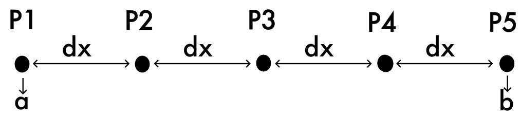
The function f(x) exists in "all space". However, the integration is bounded to the limits a to b, $I=\int_a^{b} f\left(x\right)\mathrm{d}x = \int_0^{3\pi} \left(20 \cos(x)+3x^2\right)\mathrm{d}x$.
Use those limits to create an x array using linspace(a,b,n), where a is the limit to the left, b is the limit to the right and n is the number of points. Below you see the case with 5 points.
Task 3:
Define the intervals a,b and the number of points needed to have a subinterval length $\Delta x=\pi$.
a = YOUR_CODE_HERE
b = YOUR_CODE_HERE
number_of_points = YOUR_CODE_HERE

x_values = np.linspace(YOUR_CODE_HERE)
dx = x_values[1]-x_values[0]

print("x  = ",x_values)


# test dx value
assert abs(dx - np.pi)<1e-5, "Oops! dx is not equal to pi. Please check your values for a, b and number of points."
Task 4:
How do the number of points and number of subintervals relate? Write a brief answer below.
answer:
Visualize a "continuous" function and list comprehension
For visualization purposes in the rest of the notebook, f(x) is here evaluated with high resolution. A "list comprehension" method is used for this purpose. Understanding "list comprehensions" is essential to solve the rest of the notebook.
Visualize a "continuous" function and list comprehension
For visualization purposes in the rest of the notebook, f(x) is here evaluated with high resolution. A "list comprehension" method is used for this purpose, which is a special feature of the Python programming language (you learned about it in the PA!).
Task 5:
Three equivalent solutions to define f_high_resolution are shown below. The first one loops x_high_resolution and assigns its values to x, which is then used to evaluate f.
The second one creates an index list based on the number of points contained in x_high_resolution, then loops it to evaluate f at each element of x_high_resolution.
The third simply uses a function to evaluate the values.
Which method do you find easier to read/write?
NOTE: although list comprehensions may look more cumbersome here, it is important tool to learn, as in more complex code it can help make the algorithm easier to read and write. In terms of computation time, list comprehensions are faster than "regular" for loops (both are native Python features), However, the third approach is actually the fastest in terms of numerical computation time, because Numpy ndarrays (not native Python) are optimized for efficient computation.
# To plot a smooth graph of the function
x_high_resolution = np.linspace(a, b, 50)

f_high_resolution = [ f(x) for x in x_high_resolution ] #first solution

f_high_resolution = [ f(x_high_resolution[i]) for i in range(len(x_high_resolution))] #second solution


# Plotting
plt.plot(x_high_resolution, f_high_resolution, '+', markersize='12', color='black')
plt.plot(x_high_resolution, f_high_resolution, 'b')
plt.legend(['Points evaluated','Continuous function representation'])
plt.title('Function for approximation')
plt.xlabel('x')
plt.ylabel('$f(x)$');
The Left Riemann Sum
This method approximates an integral by summing the area of rectangles defined with left points of the function:
$$I_{_{left}} \approx \sum_{i=0}^{n-1} f(x_i)\Delta x$$From now on, you will use ten points to define the function.
Let's look at the implementation of the Left Riemann sum following the same methods described in task 5. The differences are that (i) the index of the vector x ignores the last point, (ii) the multiplication by $\Delta x$ and (iii) the sum of the vector. Thus the result is not an array but a single number.
Task 6:
Scrutinize the correct implementations below. Why is it necessary to ignore the last point in x_values? What would happen if you include it?
x_values = np.linspace(a, b, 10)
dx = x_values[1]-x_values[0]

# Left Riemann summation: 1st option
I_left_riemann = sum( [f(x)*dx for x in x_values[:-1]] )  #method 1
print(f"Left Riemann Sum: {I_left_riemann: 0.3f}")

# Left Riemann summation: 2nd option
I_left_riemann = sum( [ f(x_values[i])*dx for i in range(len(x_values)-1) ] )  #method 2
print(f"Left Riemann Sum: {I_left_riemann: 0.3f}")
Task 7:
Scrutinize the correct implementation below to visualize the bar plot (plt.bar) and location of the points (plt.plot with '*', in the line code below plt.bar) that define the height of each rectangle.
Tip: The bar plot requires one less element than the total number of points defining the function.
# Visualization
# Plot the rectangles and left corners of the elements in the riemann sum
plt.bar(x_values[:-1],[f(x) for x in x_values[:-1]], width=dx, alpha=0.5, align='edge', edgecolor='black', linewidth=0.25)
plt.plot(x_values[:-1],[f(x) for x in x_values[:-1]], '*', markersize='16', color='red')

#Plot "continuous" function
plt.plot(x_high_resolution, f_high_resolution, 'b')
plt.title('Left Riemann Sum')
plt.xlabel('x')
plt.ylabel('$f(x)$');
The Right Riemann Method
Similar to the left Riemann sum, this method is also algebraically simple to implement, and can be better suited to some situations, depending on the type of function you are trying to approximate. In this case, the subintervals are defined using the right-hand endpoints from the function and is represented by
$$I_{_{right}} \approx \sum_{i=1}^n f(x_i)\Delta x$$Task 8:
Complete the code cell below for the right Riemman method..
Tip: Consult the Left Riemann implementation above as a guide.
I_right_riemann = sum( [YOUR_CODE_HERE for x in YOUR_CODE_HERE] )

print(f"Right Riemann Sum: {I_right_riemann: 0.3f}")
Task 9:
Complete the code cell below to visualize the right Riemman method.
# Right Riemann sum visualization
plt.bar(x_values[YOUR_CODE_HERE],[f(x) for x in x_values[YOUR_CODE_HERE]],
        width=YOUR_CODE_HERE, alpha=0.5, align='edge',
        edgecolor='black', linewidth=0.25)
plt.plot(x_values[YOUR_CODE_HERE],[f(x) for x in x_values[YOUR_CODE_HERE]],
         '*', markersize='16', color='red')
#Plot "continuous" function
plt.plot(x_high_resolution, f_high_resolution, 'b')
plt.title('Right Riemann Sum')
plt.xlabel('x')
plt.ylabel('$f(x)$');
Midpoint Method Approximation
For a function defined with constant steps (uniform $\Delta x$), the midpoint method approximates the integral taking the midpoint of the rectangle and splitting the width of the rectangle at this point.
$$I_{_{mid}} \approx \sum_{i=0}^{n-1} f\left(\frac{x_i+x_{i+1}}{2}\right)\Delta x $$Task 10:
Complete the code cell below to implement the midpoint sum below.
I_midpoint = sum([f(YOUR_CODE_HERE)*dx for i in range(YOUR_CODE_HERE)])
print(f"Midpoint Sum: {I_midpoint: 0.3e}")

I_midpoint = sum([f(x_at_the_middle)*dx for x_at_the_middle in YOUR_CODE_HERE ])
print(f"Midpoint Sum: {I_midpoint: 0.3e}")
Task 11:
Complete the code cell below to visualize the midpoint method.
# Midpoint sum visualization
plt.bar(x_values[YOUR_CODE_HERE],[f(x_at_the_middle) for x_at_the_middle in YOUR_CODE_HERE ], width=dx, alpha=0.5, align='edge', edgecolor='black', linewidth=0.25)
plt.plot(x_values[YOUR_CODE_HERE],[f(x_at_the_middle) for x_at_the_middle in YOUR_CODE_HERE],'*',markersize='16', color='red')
#Plot "continuous" function
plt.plot(x_high_resolution, f_high_resolution, 'b')
plt.title('Midpoint Sum')
plt.xlabel('x')
plt.ylabel('$f(x)$');
Trapezoidal Rule
This method requires two evaluations of the function $f$ for each 'rectangle', at its left and right corners. In fact, it does not represent a 'rectangle anymore' but a trapezoid. For a 1D case, it is a rectangle with a triangle on top.
$$I_{_{trapezoid}} \approx \sum_{i=0}^{n-1}\frac{f(x_i)+f(x_{i+1})}{2}\Delta x $$Task 12:
Complete the following code to implement the trapezoidal rule for the sum.
I_trapezoidal = sum([YOUR_CODE_HERE for i in range(len(x_values)-1)])
print(f"Trapezoidal Sum: {I_trapezoidal: 0.5e}")
Task 13:
To visualize the trapezoidal method a plt.bar is not used rather plt_fill_between. Revise the code cell below.
# Trapezoidal sum
for i in range(len(x_values)-1):
    plt.fill_between([x_values[i], x_values[i+1]],
                     [f(x_values[i]), f(x_values[i+1])],
                     alpha=0.5)

#Plot "continuous" function
plt.plot(x_high_resolution, f_high_resolution, 'b')
plt.title('Trapezoidal Sum')
plt.xlabel('x')
plt.ylabel('$f(x)$');
Absolute errors in integral
Task 14:
Compute the absolute errors of each method. Are they similar to your expectatations? (i.e. corresponding to the orders of magnitude).
# Calculate absolute errors
left_riemann_error = YOUR_CODE_HERE
right_riemann_error =  YOUR_CODE_HERE
midpoint_error = YOUR_CODE_HERE
trapezoidal_error = YOUR_CODE_HERE

# Print the results
print(f"Left Riemann Error: {left_riemann_error: 0.3e}")
print(f"Right Riemann Error: {right_riemann_error: 0.3e}")
print(f"Midpoint Error: {midpoint_error: 0.3e}")
print(f"Trapezoidal Error: {trapezoidal_error: 0.3e}")
Simpson's Rule
Simpson's rule is a method that uses a quadratic approximation over an interval that allows the top bound of the area 'rectangle' to be defined by a polynomial. In general, it can be a better approximation for curved, but mathematically smooth functions. It also has the requirement that subintervals must be an even number, so this is something to be aware of when using it in practise. As a sum, it is defined as
$$\int^{b}_{a}f(x)\mathrm{d}x\approx \sum_{i=1}^{n/2}\frac{1}{3}(f(x_{2i-2})+4f(x_{2i-1})+f(x_{2i}))\Delta x$$where $n$ must be an even integer.
Challenge
Take what you have seen in the other numerical implementation codes and implement Simpson's Rule for the same integral! A redefinition of x_values is done with 9 points instead of 10 as an uneven number of points is required to apply Simpson's Rule.
# Define Simpson's Rule here
x_values = np.linspace(YOUR_CODE_HERE)
dx = YOUR_CODE_HERE

simpson_integral = sum([ YOUR_CODE_HERE ])

# Calculate the absolute error
simpson_error = YOUR_CODE_HERE

# Print the result and error
print(f"Simpson's Rule Integral: {simpson_integral: 0.5e}")
print(f"Simpson's Rule Absolute Error: {simpson_error: 0.5e}")
Task 15:
Refine the number of points using the integration by left riemann until reaching a similar accuracy as for the trapezoidal rule. How much finer was your grid?
End of notebook.
